June, 2022
Dataflow is an abstract mathematical model that can be used to model repetitive deterministic operations on streams of products, or streams of data items, often including the resources on which they are realized. They are used, for instance, to model applications on processor platforms, to model manufacturing systems, or train schedules.
A timed dataflow graph consists of
Actors from \(A\) represent the activities in the model. An actor can fire, which means that it executes its activity. Actors can fire repetitively and indefinitely, unless there are constraints that prevent it. The firings of an actor have a fixed duration given by the function \(e\) and multiple firings of the same actor can be ongoing simultaneously. A channel \(({a_1},n,{a_2})\) is a dependency of the firings of actor \({a_2}\) on the firings of the actor \({a_1}\). The firing number \(k+n\) of actor \({a_2}\) cannot start before firing number \(k\) of \({a_1}\) is complete. There is no dependency for the first \(n\) firings of \({a_2}\). An input dependency \(d_I(i)={a}\) means that firing \(k\) of actor \({a}\) depends on the presence of input number \(k\) on input \(i\). Output dependency \(d_O(o)={a}\) means that output number \(k\) on output \(o\) is produced by firing \(k\) of actor \({a}\).
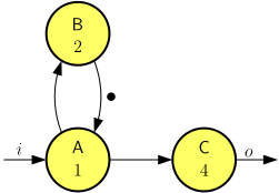
Figure 1 shows an example of an SDF model. The circles in the figure are the actors. In a representation of an SDF graph, we often give actors a name. In Figure 1, the names are written inside the actors A, B, C. The durations of the firings are also written inside the actor. For instance, the firings of actor C take 4 time units each. Arrows between actors represent the channels. For example, the channel from A to C creates the constraint that firing number \(k\) of actor C cannot start before firing number \(k\) of A is complete. This can be described operationally as if actor A produces an output token onto the channel every time it completes a firing and actor C consumes a token when it starts its firing. We often use this operational view when it is more convenient. The channel from B to A has an initial token, even before B has completed any firings. Without it a cyclic dependency would prevent actors A and B from ever firing.
The graph has one input \(i\). The input dependency is shown by an arrow from the input to the actor that depends on it. The graph has one output \(o\). The output dependency is shown by an arrow from the actor that produces it to the output.
If we assume that the first firings start at time \(0\) and further all actor firings start as soon as allowed by the constraints, then behavior including the first four firings of each actor is shown in Figure 2 in the form of a Gantt chart. The horizontal axis is a time line. On the first row, the arrival of the four inputs is shown with dots at the points in time when they arrive. Actor A is the first to fire when the first input, on which it depends, arrives. Actors B and C follow with their first firings when A completes its first firing. Observe that the firings of B and C occur in parallel. Observe also that the firings of actor C overlap. For instance, its second firings starts at time 5, while its first firing only ends at time 6. The last row shows the outputs produced by actor C onto output \(o\). They coincide with the completions of the firings of C.
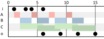
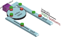
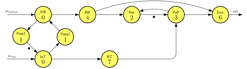
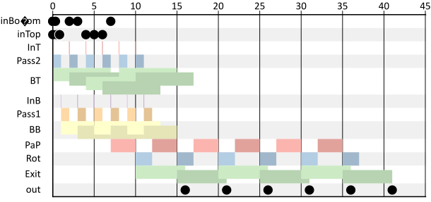
Figure 3 shows a simple manufacturing system. It takes two kinds of objects on the input conveyor belt. We call those types of objects ‘bottoms’ (shown as red objects) and ‘tops’ (shown as green objects) and the purpose of the system is to combine them into a combined product by placing the tops on the bottoms. The bottoms and tops are fed into the system alternatingly, starting with a top. Tops are transported by conveyor belts to a pick-and-place unit. Bottoms are transported on the conveyor belt to a rotating indexing table, which will rotate it towards the pick-and-place unit that will place the top on top of it. The combined product is transported by the indexing table to another conveyor belt, which will move the object to the system output. The indexing table always simultaneously rotates a new bottom to the pick-and-place unit and the combined product to the belt. Therefore, at startup of the system, a bottom part is initially placed on the indexing table at the pick-and-place unit.
Figure 4 shows a dataflow model of this manufacturing system. It has two inputs, \(\mathit{in}_{\mathit{bottom}}\) and \(\mathit{in}_{\mathit{top}}\) representing the arrivals of bottoms and tops, respectively. Tops and bottoms are admitted onto the conveyor belt alternatingly. This is modeled by the cycle of actors InT—Pass2—InB—Pass1. InB fires when a new bottom is admitted and InT when a top is admitted. This happens when the object is available and the belt is clear. Actors Pass1 and Pass2 model the time it takes after admission of an object to clear the belt for another object. The initial token on the cycle ensures that the first object admitted is a top.
The sequence of actors at the top of the figure follows the operations applied to the bottoms. Actor BB models its transport to the indexing table. Rot models its rotating on the table towards the pick-and-place unit. PaP models the pick-and-place unit placing a top on it. Exit models the final transport towards the output including the rotation on the index table and the transport on the belt to the output. The BT actor models the transport of the top on the belt to the pick-and-place unit, where it is combined with a bottom.
Most dependencies in the graph are straightforward. The initial token on the channel from Rot to PaP represents the bottom part that is initially placed in the system. The dependency from PaP to Rot ensures that the indexing table does not rotate until the pick-and-place operation is complete. The dependency from BB to Exit ensures that the second rotation is correctly modelled. It only starts when a new bottom part is ready to move onto the indexing table.
Figure 5 shows a Gantt chart of the behavior of the manufacturing system. Note that the arrivals of tops and bottoms are arbitrary, but early enough to not impact the schedule. Observe the cycle of firings of InT, Pass2, InB and Pass1 as the objects are admitted to the system. The firings of the BT and BB actors overlap, as multiple objects are transported on the same conveyor belt simultaneously. Rot and Exit always start simultaneously as they both capture the rotating of the indexing table. Completed products appear at the output starting from time \(16\) periodically with \(5\) time units in between. It appears that the critical path for producing the outputs is formed by the alternating PaP and Rot actors.
The timed dataflow models we have introduced are sometimes also called single-rate dataflow models. There are also multi-rate timed dataflow models. In a multi-rate dataflow graph, actor firings may produce and/or consume multiple tokens with every firing. This rate must however be constant, i.e., every firing of the same actor always produces and consumes the same quantity of tokens. The number \(c\in\mathbb{N}\), \(c>0\) of tokens it consumes from an input channel is called the consumption rate and the number \(p\in{}\mathbb{N}\), \(p>0\) of tokens it produces is called the production rate.
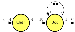
As an example, consider the cleaning and boxing of eggs. The cleaning machine takes four eggs at a time and a packing machine packs ten eggs at a time in a box. The inputs are eggs and the outputs are boxes of ten eggs. This can be modelled with the following multi-rate dataflow graph.

Firings of the Clean actor require four eggs from the input to be enabled and produce four clean eggs every time they complete. Firings of the actor Box require ten eggs to be produced by Clean to be enabled. In figures, we write the production rates as a number at the producing end of a channel and the consumption rates at the consuming end of a channel.
In single-rate dataflow graphs dependencies between actors are one-to-one. In multi-rate dataflow graphs they can be one-to-one, many-to-one, one-to-many or many-to-many, depending on the production and consumption rates. However, because the production and consumption rates are constant, it is possible in a well-behaved multi-rate dataflow model to find a number of firings for each of the actors, i.e., a mapping \(\rho{}: A\rightarrow\mathbb{N}\), such that \(\rho{}(a)>0\) for all \(a\in{}A\), and for every channel from actor \(a\) with production rate \(p\) to actor \(b\) with consumption rate \(c\) in the graph, the following equation, called the balance equation holds. \[ \rho{}(a)\cdot{}p = \rho{}(b)\cdot{}c \]
The equation states that with a collection of firings according to the numbers in \(\rho{}\) for every channel, the production of tokens onto the channel and the consumption of tokens from the channel are balanced, i.e., equal. For the example of the eggs, such a solution exists, \(\rho{}(Clean)=5\) and \(\rho{}(Box)=2\). The unique, smallest solution \(\rho{}\) is called the repetition vector of the multi-rate dataflow graph. \(\rho{}(Clean)=25\) and \(\rho{}(Box)=10\) is also a solution to the balance equations, but it has more firings than necessary to be balanced. A collection of firings according to the repetition vector is together called an iteration of the graph.
A multi-rate graph that does not have a repetition vector cannot have a balanced production and consumption of tokens and is not well-behaved. It is called inconsistent. The graph below, for example, is inconsistent. For any \(\rho{}(Box)>0\), \(\rho{}(Box)\cdot{}3 \neq \rho{}(Box)\cdot{}2\). In terms of the operational interpretation, more and more tokens would accumulate on the channel over time, which does not represent meaningful behavior.
If a repetition vector does exist, the graph is called consistent.
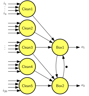
We will not present a precise mathematical definition of the constraints of a multi-rate dataflow graph. Instead, we show how a consistent multi-rate dataflow graph with repetition vector \(\rho{}\) can be converted to a single-rate dataflow graph.
The conversion proceeds by creating \(\rho{}(a)\) single-rate actors for every actor \(a\) in the multi-rate graph. The graph below shows the single-rate version of the graph above. There are \(\rho{}(Clean)=5\) ‘copies’ of the actor Clean en \(\rho{}(Box)=2\) actors for the actor Box. The first firing of the original actor Clean will be represented by the first firing of the new actor Clean1, the second firing of Clean will be represented by the first firing of the new actor Clean2, and so on. The dependencies between firings are reconstructed by new channels, for example, the firing of Box1 needs ten eggs, which are produced (4+4+2) by the first three firings of Clean and thus it depends on Clean1, Clean2 and Clean3. Similarly, Box2 depends on Clean3, Clean4 and Clean5. The sixth firing of Clean can then be represented by the second firing of Clean1, because \(\rho{}\) satisfies the balance equations, and so on. Note how the self-edge of the Box actor has been converted to a loop between Box1 and Box2. The original channel represents a dependency of firing \(k\) of Box on firing \(k-1\). After the conversion firing \(k\) and firing \(k-1\) are represented by different actors. Had the original channel two initial tokens, the dependency would be between firing \(k\) and firing \(k-2\), which are represented by the same actor after conversion. In that case, actors Box1 and Box2 would both have had a self-edge with one initial token. Further, to comply with the single-rate inputs, we now need to distribute (in the model, not on the farm) the 20 eggs among 20 inputs, and similarly the output boxes are split.
Consider the following dataflow graph, which provides a simple model of a Wireless Channel Decoder (WCD).
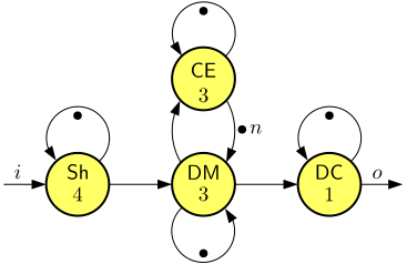
The WCD has an input \(i\) over which it receives modulation symbols and an output \(o\) through which it outputs decoded data. The Shift actor Sh maintains synchronization with the transmitter, the DM actor DeModulates the incoming signal, the CE actor Estimates the radio Channel, and the DC actor DeCodes the symbol. Channel estimation and decoding may be done in parallel. The number of tokens on the channel from the channel-estimation actor CE to the demodulation actor DM determines how old the channel-estimation information is that DM uses. If \(n=1\), then DM uses information based on the previously received symbol. If \(n=2\), it uses information that is two symbols old.
Consider a simple producer-consumer pipeline consisting of a Producer actor P, a Filter actor F, and a Consumer actor C. Any produced sample is first filtered and then consumed again. Assume that the producer actor has an execution time (firing duration) of 2 time units to produce one sample and that the consumer actor has an execution time of 1 time unit per sample. The execution time of F varies based on the function being applied. With function \(f_1\) it has an execution time of 1; with \(f_2\), it has an execution time of 3. Samples are produced and consumed one at a time, but the filtering of multiple samples may occur in parallel. The producer and the consumer are coupled to the filter with two buffers, each having space for two samples. Initially, the two buffers are empty. An actor claims space for producing an output sample into a buffer at the start of firing; it releases space of a consumed sample at the completion of firing.
Consider the following dataflow graph modeling a simple Image-Based Control (IBC) pipeline.
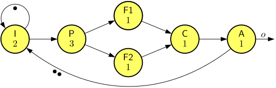
The pipeline has two actors, I and P, that capture an Image and Process it to extract two features. These two Features are processed by actors F1 and F2. Based on the features the pipeline computes a Control action in Actor C and eventually actuates the controlled plant with Actor A through output \(o\). The model illustrates IBC pipelines as are used in, for example, autonomous vehicles. Note that the I actor with a channel to itself (a self-loop) with one initial token models a periodic image source with period 2.
We define the average actuation rate as the average number of outputs over time, ignoring any initial start up behavior in which the number of actuation actions may be lower. We define the actuation delay as the time between the start of an I firing and the corresponding \(o\) actuation output.
The next step is to implement the (optimized) IBC pipeline. Assume actors I, P, C, and A are each mapped onto their own processor that executes an actor firing with the given execution time. Assume actors F1 and F2 are scheduled together on a processor, where firings take one time unit and are scheduled alternatingly, starting with an F1 firing. The implemented IBC pipeline is referred to as the IBC System (IBCS). The IBCS should operate at the maximum output rate derived earlier.
Consider the following Gantt chart of a Video Decoder (VD) pipeline.
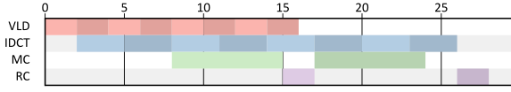
The Variable-Length Decoding actor VLD decodes macroblocks of an incoming video frame, the IDCT actor performs an Inverse Discrete Cosine Transform on a macroblock, the MC actor performs Motion Compensation, and the ReConstruct actor RC composes a frame from the decoded macroblocks.
Consider again the Image-Based Control System (IBCS) of Exercise 3. We continue with the further development of the optimized system given in the answer to the last item of that exercise. Assume the processing actor P is adapted to an actor P+ that extracts four extra features of a different type than the original two features. These new features can be processed twice as fast as the original features on a normal processor, by an actor FF (for Fast Features), where each firing processes one feature. Also the actor that computes the control action is updated, to C+, to include the information of the new features. So it uses both the four new features and the two earlier ones.
(Hint: Check the correctness of your models by comparing the Gantt charts of the two models in the CMWB.)
We now create a variant of the IBCS in which the workload of the feature processing is distributed equally over processors P3 and P4. Each processor receives two fast features and one of the original features. Each of the processors hosts a copy of the FF and F actors. Each processor first processes the two fast features and then the slow feature.