June, 2022
We often consider sequences of events. For instance, a sequence of (arrivals of) products that need to be manufactured, or a sequence of data items that need to be processed. Such sequences have a beginning, but do not need to have an end, i.e., they can be of finite length \(n\in\mathbb{N}\), or they can be of infinite length. For performance analysis purposes, mathematically, we refer to sequences of time stamps of events. We call them, in short, event sequences. We denote sequences of events by lower case letters and we use parentheses to refer to the events in a sequence. \(s(k)\) with \(k\geq 0\) denotes event number \(k\) in event sequence \(s\). If \(s\) is finite and has length \(n\), then \(s(k)\) is not defined for \(k\geq{}n\). We refer to \(k\) as the event index.
An event sequence \(s\) is a function \(s: \mathbb{I}\rightarrow \mathbb{T}\), where \(\mathbb{I}=\{0, \ldots{}n-1 \}\) for a finite sequence of length \(n\) and \(\mathbb{I}=\mathbb{N}\) for an infinite sequence.
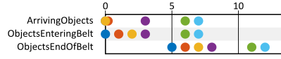
We illustrate event sequences, as shown in Figure 12, by a time line with a row of dots at the time stamps of the events. Event indices are indicated by colors of the dots. Note that events in an event sequence do not necessarily have non-decreasing time stamps, i.e., it may be the case that \(s(k) > s(k+1)\). Where needed, we use the following color coding to represent the event index, i.e., event with index 0 is blue, 1 is orange, 2 is yellow, 3 purple, etcetera.
We define the following operations on event sequences, because we need them later.
If \(s\) is an event sequence, then \({{s}^{N}}\) is the event sequence such that \({{s}^{N}}(k) = -\infty{}\) if \(k<N\) and \({{s}^{N}}(k) = s(k-N)\) if \(k\geq{}N\). If \(s\) is of finite length \(n\) then \({{s}^{N}}\) is a finite event sequence of length \(n+N\). If \(s\) is infinite, then \({{s}^{N}}\) is infinite.
Let \(s_1\) and \(s_2\) be two event sequences of the same length. Then \(s_1\oplus{}s_2\) is an event sequence, also of the same length, such that \((s_1\oplus{}s_2)(k) = s_1(k)\oplus{}s_2(k)\).
Let \(s\) be an event sequence and \(c\in{}\mathbb{T}\). Then \(c\otimes{}s\) is an event sequence, of the same length, such that \((c\otimes{}s)(k) = c\otimes{}s(k)\).
We use \(\epsilon{}\) to denote the infinite event sequence with \(\epsilon{}(k)=-\infty{}\) for all \(k\in\mathbb{N}\).
The \(\mu{}\)-periodic event sequence is the infinite event sequence \(s\) with \(s(k)=\mu{}\cdot{}k\) for all \(k\in\mathbb{N}\).
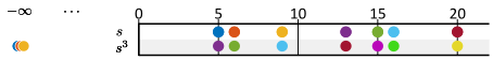
Figure 13 shows an event sequence \(s\) and the event sequence \(s^3\) which is delayed by 3 samples. Note that the time stamps are the same, except for the added time stamps of \(-\infty{}\), which are not visible on the time line. The indices have changed, as can be observed from the modified colors. For example, \({{s}^{3}}(4)=s(1)=6\).
We use the following notation for event sequences: \[ s=[t_0, t_1, t_2, \ldots{}] \]
In this case, \(s\) is the event sequence such that \(s(0)=t_0\), \(s(1)=t_1\), \(s(2)=t_2\), etcetera.
We use event sequences to study the performance of systems. We therefore define their throughput as follows.
If \(s\) is an infinite event sequence, then the throughput of \(s\) is given by the following limit, if it exists: \[ \tau{}(s) = \lim_{k\rightarrow{}\infty{}} \frac{k}{s(k)} \]
The throughput of the \(\mu{}\)-periodic event sequence, for example, is \(\frac{1}{\mu{}}\).
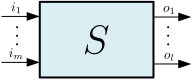
We are interested in systems that operate on one or more sequences of events. A system takes a number of input event sequences and produces one or more output event sequences. We consider systems that are deterministic. The output sequences are uniquely determined by the input sequences. If a system \(S\) produces for input sequences \(i_1, \ldots{}, i_m\) the output sequences \(o_1\ldots{}, o_l\), we write \[i_1, \ldots{}, i_m \mathbin{\stackrel{S}{\longrightarrow}} o_1\ldots{}, o_l\]
A visualization is shown in Figure 14.
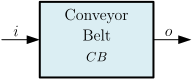
The conveyor belt from Example 7 can be described as an event system if we assume that it has a (finite or infinite) input sequence of objects arriving that need to be transported in a given order along the conveyor belt. It is visualized in Figure 11 as an abstract box \(CB\) with input \(i\) and output \(o\). The system has a single output, the arrival events of the objects at the end of the conveyor belt. The output sequence is equally long as the input sequence, all boxes arrive at the end of the belt. It is also deterministic, following the equations presented in Example 7.
We consider a class of event systems that have special properties. We look at properties that are akin to the classical concept of linear time-invariant systems (LTI systems).
An event system \(S\) is called max-plus-linear if for all event sequences \(i_k\), \(j_k\), \(o_k\), \(p_k\), and any \(c\in\mathbb{T}\), the following properties hold:
An event system \(S\) is called index invariant if for all event sequences \(i_k\), \(o_k\), and any \(N\in\mathbb{N}\), the following property holds:
Additivity of an event system means that if a set of input sequences corresponds to the point-wise maximum of two (or more) input sequences, then the corresponding output, similarly, corresponds to the point-wise maximum of the individual outputs. This allows us to break down complex input sequences into smaller parts and analyze them separately, both along the different input sequences to the system and to the individual events in those sequences.
Homogeneity means that the system is insensitive to absolute time of the various events; it is sensitive only to the relative time differences. If we shift all inputs backward or forward by a fixed amount of time, then also all outputs will shift by the same amount of time. This property allows us to perform some analysis for an arbitrary absolute point in time and translate the results to other points in time.
Similarly, index-invariance allows us to limit our analysis to a given event index and translate the analysis results straightforwardly to other event indices.(This is a good moment to reconsider Exercise 9.)
In Example 7 we have concluded the following equation to describe the conveyor belt event system \(o\mathbin{\stackrel{CB}{\longrightarrow}}a\). (Note that in Example 7 we started counting objects from 1 and the indices of event sequences start from 0.) \[ a(n) = \bigoplus_{0\leq{}k<n}\frac{l+(n-1-k)d}{v}\otimes{} o(k) \]
(additivity) Let \(o_1 \mathbin{\stackrel{CB}{\longrightarrow}} a_1\), \(o_2 \mathbin{\stackrel{CB}{\longrightarrow}} a_2\) and \(o_1\oplus{}o_2 \mathbin{\stackrel{CB}{\longrightarrow}} a_3\). Then \[ \begin{aligned} a_3(n) &= \bigoplus_{0\leq{}k<n}\frac{l+(n-1-k)d}{v}\otimes{} (o_1\oplus{}o_2)(k) \\ &= \bigoplus_{0\leq{}k<n}\frac{l+(n-1-k)d}{v}\otimes{} o_1(k) \oplus{} \frac{l+(n-1-k)d}{v}\otimes{} o_2(k)\\ &= \left(\bigoplus_{0\leq{}k<n}\frac{l+(n-1-k)d}{v}\otimes{} o_1(k)\right) \oplus{} \\ & \hspace{1.0cm} \left(\bigoplus_{0\leq{}k<n} \frac{l+(n-1-k)d}{v}\otimes{} o_2(k)\right)\\ &= a_1(n) \oplus{} a_2(n)\\ \end{aligned} \]
Thus, \(o_1\oplus{}o_2\mathbin{\stackrel{CB}{\longrightarrow}}a_1\oplus{}a_2\)
(homogeneity) Let \(o \mathbin{\stackrel{CB}{\longrightarrow}} a\), and \(c\otimes{}o \mathbin{\stackrel{CB}{\longrightarrow}} a'\). Then \[ \begin{aligned} a'(n) &= \bigoplus_{0\leq{}k<n}\frac{l+(n-1-k)d}{v}\otimes{} (c\otimes{}o)(k) \\ &= \bigoplus_{0\leq{}k<n} c\otimes{} \frac{l+(n-1-k)d}{v}\otimes{} o(k) \\ &= c \otimes{} \bigoplus_{0\leq{}k<n} \frac{l+(n-1-k)d}{v}\otimes{} o(k) \\ &= c\otimes{}a(n)\\ \end{aligned} \]
Thus, \(c\otimes{}o\mathbin{\stackrel{CB}{\longrightarrow}}c\otimes{}a\)
(index invariance) Let \(o \mathbin{\stackrel{CB}{\longrightarrow}} a\) and \({{o}^{N}} \mathbin{\stackrel{CB}{\longrightarrow}} a'\). Then \[ \begin{aligned} a'(n) &= \bigoplus_{0\leq{}k<n}\frac{l+(n-1-k)d}{v}\otimes{} ({{o}^{N}})(k) \\ &= \left(\bigoplus_{0\leq{}k<N}\frac{l+(n-1-k)d}{v}\otimes{} -\infty{}\right)\oplus{} \\ & \left(\bigoplus_{N\leq{}k<n}\frac{l+(n-1-k)d}{v}\otimes{} o(k-N)\right) \\ &= \left(\bigoplus_{N\leq{}k<n}\frac{l+(n-1-k)d}{v}\otimes{} o(k-N)\right) \\ & \{\text{substitute}~~m=k-N\}\\ &= \bigoplus_{0\leq{}m<n-N}\frac{l+(n-1-(m+N)))d}{v}\otimes{} o(m) \\ &= \bigoplus_{0\leq{}m<n-N}\frac{l+((n-N)-1-m))d}{v}\otimes{} o(m) \\ &= \left\{ \begin{array}{cl} -\infty{} & \textrm{if} ~~ n< N\\ a(n-N) & \textrm{if} ~~ n\geq N\\ \end{array} \right.\\ &= {{a}^{N}}(n)\\ \end{aligned} \]
Thus, \({{o}^{N}}\mathbin{\stackrel{CB}{\longrightarrow}}{{a}^{N}}\)
Dataflow graphs can be seen as event systems by considering the token sequences arriving on inputs and produced on outputs as event streams. Dataflow graphs are, in general, not necessarily linear systems though, since their behavior is only determined with a schedule. As we will see later, however, our primary interest is in self-timed schedules of dataflow graphs. Assuming the availability of initial tokens at the earliest possible point in time, \(-\infty{}\), and hence no artificial lower bound, 0 or otherwise, on the firing times, the self-timed schedule is uniquely determined by the input sequences. Actor firings that do not depend on any input then start (and complete) at time \(-\infty{}\). As a result, a self-timed dataflow graph is deterministic and dataflow graphs with self-timed execution are linear and index-invariant systems.
A single-rate dataflow graph under self-timed execution and with initial tokens available at \(-\infty{}\) is a linear and index-invariant system.
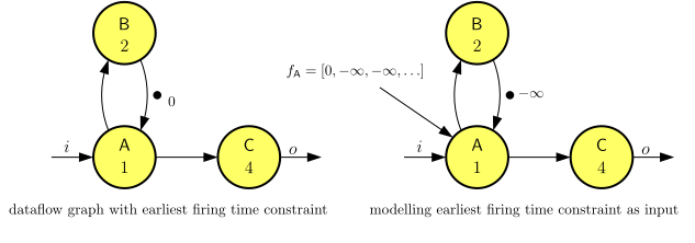
Theorem 3 appears to restrict the application of properties of index-invariant systems to dataflow graphs to which no additional constraints have been applied on the earliest firing times, or to the availability of initial tokens. Indeed, such dataflow graphs need not be index-invariant. However, we can alternatively model the additional constraints by additional inputs, allowing the system to be modelled as an index-invariant system including the analysis opportunities this offers. Figure 15 shows the dataflow graph of Figure 1, with the applied constraint that actors cannot fire earlier than time stamp 0. This is indicated by the time stamp \(0\) label next to the initial token in the graph. This restricts actor A to not fire before time 0 and in this example that ensures that also other actors cannot fire before time 0. This behavior can also be modelled with the graph on the right hand side of the figure. This graph has no additional constraints on firing times, indicated by the time stamp of \(-\infty{}\) on the initial token. There is however, an additional input added to actor A. The firing constraints can be enforced by applying the right input sequence to input \(f_{A}\). The input sequence \(f_{A}=[0, -\infty{}, -\infty{}, -\infty{}, \ldots]\) enforces that no actor firing occurs before time 0, the equivalent of the graph on the left of the figure. Such an input can also be used to enforce other constraints. For example. \(f_{A}=[0, 5, 10, 15, \ldots]\) restricts A to (not fire earlier than) a periodic schedule. Using this approach to model additional firing constraints Theorem 2 applies to such dataflow graphs and analysis methods, introduced later, that depend on it can be applied.
Multi-rate dataflow graphs are also linear, i.e., satisfy both the additivity and homogeneity properties. They are however not index invariant. Since their actors consume and/or produce multiple tokens at a time, input events with different indices may encounter different actor firings leading to different, not just shifted, output sequences. In the multi-rate example of the eggs, for instance, the second egg ends up in the same output box as the first egg, not the second box as index invariance would require.
We have seen, however, that a multi-rate graph can be converted to a single-rate graph, which is index invariant. In case of the eggs, it has twenty (egg) inputs and two (box) outputs. This means that if we shift by twenty input events and two output events, the response is invariant.
In general, multi-rate dataflow graphs do obey a property that is similar to index invariance, but it requires the indices to be shifted in accordance with a multiple of the repetition vector.
Reconsider the fragment of the Wireless Channel Decoder (WCD) dataflow model of Exercise 9. Show that this dataflow graph models a max-plus-linear index-invariant event system. For the purpose of this analysis, consider the arrival/production times on the inputs resp. output as event sequences. You may assume that the event sequence corresponding to the production times of tokens on the self-loop of Actor Sh is \((4\otimes i)^1\), when \(i\) is the event sequence corresponding to the input channel \(i\) and \(\_^1\) is the delay operator of Definition 10. (The observant reader may notice that this assumption is only valid if inputs on channel \(i\) arrive with intermediate arrival times of at least 4. We come back to this aspect in later exercises.)
If a system is linear then we can apply a divide-and-conquer strategy to analyze how it responds to complex stimuli. For example, the manufacturing system of Example 2 is a max-plus-linear event system. \[ \mathit{in}_{\mathit{top}}, \mathit{in}_{\mathit{bottom}} \mathbin{\stackrel{MS}{\longrightarrow}} o\]
Additivity says that if \(\mathit{in}_{\mathit{top}}, \epsilon{} \mathbin{\stackrel{MS}{\longrightarrow}} o_1\) and \(\epsilon{}, \mathit{in}_{\mathit{bottom}} \mathbin{\stackrel{MS}{\longrightarrow}} o_2\), then \(o= o_1\oplus{}o_2\).
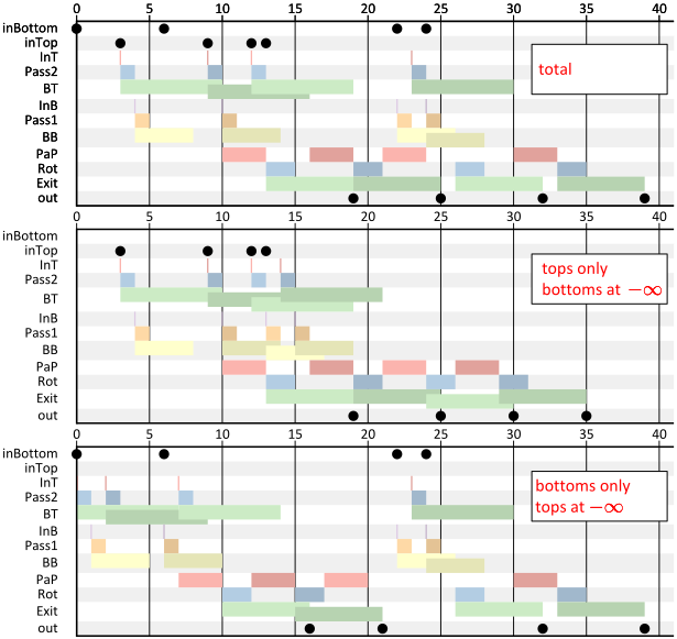
Assume that \(\mathit{in}_{\mathit{bottom}} = [0, 6, 22, 24]\) and \(\mathit{in}_{\mathit{top}}= [3, 9, 13, 12]\). Figure 16 shows the response of the system to \(\mathit{in}_{\mathit{top}}, \mathit{in}_{\mathit{bottom}}\), to \(\mathit{in}_{\mathit{top}},\epsilon{}\) and to \(\epsilon{}, \mathit{in}_{\mathit{bottom}}\). It is easy to verify that the output in the first case is indeed the maximum of the two output sequences of the second and the third case. In fact, observe that it is true for the entire Gantt chart that for any actor firing, the starting time is the maximum of the two starting times in the bottom two cases, and therefore also equal to at least one of the two cases. This is to be expected since one could consider those events to be observable outputs of the event system, for which the same property should hold.
This property is often referred to as the and can be effectively used to simplify the analysis of the response of a system to a complex combination of stimuli.
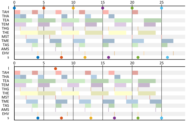
The railroad network of Example 5 can be seen as an event system if the inputs to the system are trains that are arriving from Liège. Trains departing from Maastricht need to wait for them to depart. The outputs of the system are trains arriving at the station Schiphol. The railroad network is a max-plus-linear index-invariant system since it is modelled as a dataflow graph. We can therefore apply the superposition property to study the impact of individual events in an event sequence. Assume that the top graph in Figure 17 represents the regular schedule of the trains according to the inputs \[ l = [0, 5, 10, 15, 20, 25] \]
As outputs of the system, assuming self-timed execution with trains (tokens) \(T_1\) through \(T_4\) available at time 0, trains are arriving at Schiphol according to the sequence \[ s = [4, 8, 12, 16, 21, 26] \]
Imagine that we are informed that the second train from Liège, scheduled for 5.00hrs will instead arrive, delayed, at 7hrs. We now want to predict how many of the trains to Schiphol are impacted by this delay. We find the simplest event sequence \(d\) such that \(l_d=l\oplus{}d\) corresponds to the delayed event sequence. The only event that has changed is \(l(1)\), so we can take \[ d= [-\infty{}, 7, -\infty{}, -\infty{}, -\infty{}, -\infty{}]\]
and determine the response of the system to input \(d\). This response is shown in the bottom part of Figure 17. The real arrivals at Schiphol will be according to the maximum of both sequences \(l\) and \(d\). We can see that the third and the fourth train at Schiphol will be delayed by one hour. The trains after that will arrive at their scheduled times.
Consider the dataflow model of the running example of the manufacturing system of Example 2 as a max-plus-linear event system.