June, 2022
In the previous sections we have introduced timed dataflow models and their schedules and performance metrics to study timed deterministic discrete-event systems. To develop methods for performance analysis, in this module, we introduce an algebra which will help us to perform the required analysis.
To track the evolution of a system in time we label events (for example, the start of a firing, or operations in a schedule) with time stamps, real-valued numbers that indicate at what point in time an event occurs. Events can happen at any (real-valued) point in time. They can also have negative time stamps.
A time stamp is a value from the set \(\mathbb{R}\cup\{-\infty{}\}\). We denote the set of time stamps as \(\mathbb{T} \stackrel{\mathrm{def}}{=}\mathbb{R}\cup\{-\infty{}\}\).
Note that in the mathematical definition of a time stamp we also allow a time stamp to have the peculiar special value \(-\infty{}\). (Note that \(-\infty{}\notin\mathbb{R}\) and neither is \(\infty{}\), which is also not in \(\mathbb{T}\).) We will see later that this is a very convenient mathematical abstraction. In the real world events do not occur at time \(-\infty{}\)! But \(-\infty{}\) is earlier than any ‘real’ time stamp.
Consider a single-rate dataflow actor \({a}\) having a firing duration \(d=e({a})\), with a single input channel \({i}\) and a single output channel \({o}\). Assume that we know the time stamp \(x_i\) of the arrival-event of the input token to channel \({i}\). Then, we can easily compute the time stamp \(x_o\) of the production-event of the output token produced on \({o}\) when the actor \({a}\) completes its self-timed firing: \[ x_o = x_i + d \]
Now, assume that the actor \({a}\) has two input channels, \({i_1}\) and \({i_2}\). A firing of \({a}\) consumes one token from each of its inputs. We can again compute the time stamp of the production of the output token from the time stamps of the input tokens if \({a}\) fires in a self-timed manner. Recall that the self-timed execution means that the actor fires as soon as both tokens are present. If we consider the start of the firing of \({a}\) as an event with time stamp \(x_{{a}}\), then \[ x_{{a}} = \max(x_{i_1}, x_{i_2}) \] and \[ x_o = x_{{a}} + d = \max(x_{i_1}, x_{i_2}) + d = \max(x_{i_1}+d, x_{i_2}+d) \]
The very simple Example 6 illustrates that the behavior of a timed dataflow graph can be described in terms of the time stamps of the events that occur in the model and that the two important mathematical operations that describe this behavior are the \(\max\) operation and the \(+\) operation.
The operations work on time stamps from \(\mathbb{T}\) as defined in Definition 7. A mathematical definition of the algebra of the set of time stamps with the addition and maximum operations is given in Definition 8. We introduce two new symbols for the operations, because they are commonly used in literature and they are more convenient to write than the conventional notation, especially for \(\max\). Observe also that we must then define how the operators work on the special time stamp \(-\infty{}\), for which the common addition and maximum operations are not defined. The way they are defined to work on \(-\infty{}\) is however in line with our ‘intuition’ about \(-\infty{}\).
Max-plus algebra is the algebra \(\left(\mathbb{T}, \oplus{}, \otimes{}\right)\). It works on the set \(\mathbb{T}\) of time stamps and includes the operators \(\oplus{}\) and \(\otimes{}\), which are defined as follows. \[ x\oplus{}y = \left\{ \begin{array}{ll} x & \textrm{if}~~ y=-\infty{}\\ y & \textrm{if}~~ x=-\infty{}\\ \max(x, y) & \textrm{if}~~ x, y\in \mathbb{R}\\ \end{array} \right. \] \[ x\otimes{}y = \left\{ \begin{array}{ll} -\infty{} & \textrm{if}~~ x=-\infty{} ~~\textrm{or}~~ y=-\infty{} \\ x+y & \textrm{if}~~ x, y\in \mathbb{R} \\ \end{array} \right. \]
The operators of max-plus algebra have the following properties.
The symbols, \(\otimes{}\) and \(\oplus{}\) for the addition and \(\max{}\) operators are not selected arbitrarily. We can observe that the algebraic properties of max-plus algebra as introduced above are almost identical to the properties of the algebra of real numbers with the operators \(\times{}\) and \(+\) that we are all very familiar with. In the analogy, the following correspondences hold
The analogy helps us to get acquainted with the new algebra using familiarity with the traditional algebra. Check that the algebraic rules and properties mentioned above for max-plus algebra all remain valid under this correspondence.
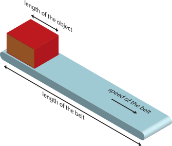
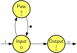
A conveyor belt (see Figure 9) is used to transport objects from one site to another, as quickly as possible. The length of the belt is \(l\) and it moves with a velocity \(v\). The objects that are transported have a size of \(d\). Three objects arrive at the time stamps: \(o_1\), \(o_2\), \(o_3\). The order of arrival is unknown, but the objects need to be transported in order (1, 2, 3). We derive max-plus-algebraic equations for the time stamps of the arrival events, \(a_1\), \(a_2\) and \(a_3\), of the three objects at the end of the belt. The first object is independent of the others, arrives at time \(o_1\), takes \(\frac{l}{v}\) time units for transportation, so it arrives at \[a_1 = o_1 + \frac{l}{v} = \frac{l}{v}\otimes{}o_1 .\]
Note that we think of \(\frac{l}{v}\) as a constant and \(o_1\) as a variable, and therefore it is more natural to write \(\frac{l}{v}\otimes{}o_1\) than \(o_1\otimes{}\frac{l}{v}\), although they are identical, just like in regular algebra we prefer to write \(3\cdot{}x\) over \(x\cdot{}3\).
The second object cannot occupy the same space on the belt and needs to be transported second. The belt is clear for the second object \(\frac{d}{v}\) time units after the arrival of object 1. So, the second object is put on the belt when the belt is clear, or, when the second object arrives, whichever is later. We can derive that the arrival at the end of the belt occurs at time \[ a_2 = \max(o_1+\frac{d}{v}, o_2) + \frac{l}{v} = \frac{l}{v}\otimes{} (\frac{d}{v}\otimes{}o_1 \oplus{} o_2) = \frac{l+d}{v}\otimes{} o_1 \oplus{} \frac{l}{v}\otimes{}o_2. \]
With similar reasoning, the third object can be shown to arrive at time \[ a_3 = \frac{l+2d}{v}\otimes{} o_1 \oplus{} \frac{l+d}{v}\otimes{} o_2 \oplus{} \frac{l}{v}\otimes{}o_3 \]
It is then also not difficult to generalize the result for more than three objects to object \(n\) arriving at time \[ a_n = \bigoplus_{1\leq{}k\leq{}n}\frac{l+(n-k)d}{v}\otimes{} o_k \]
Note that we use the \(\bigoplus{}\) notation to represent repeated application of the \(\oplus{}\) operator in the same way that the familiar \(\sum{}\) notation is used for repeated application of the \(+\) operator.
Consider the following fragment of the Wireless Channel Decoder (WCD) dataflow model of Exercise 1.
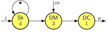
We want to analyze how the output production times depend on the input arrivals and the availability of channel-estimation information. The WCD fragment is a dataflow graph with two inputs, the symbol input \(i\) and the channel-estimation input \(ce\). Executing the dataflow model gives a sequence of token production times on symbol output \(o\), referred to as \(x_o(0), x_o(1), \ldots\). Those token production times depend on the arrival times of tokens on the inputs \(i\) and \(ce\), denoted \(x_i(0), x_i(1), \ldots\) and \(x_{ce}(1), x_{ce}(2), \ldots\), respectively. Assume that the initial token is available at time 0 and that inputs do not have negative arrival times.