by Marc Geilen (m.c.w.geilen@tue.nl); exercises by
Twan Basten
June, 2022
Answers to Exercises
Exercise
1 (A wireless channel decoder –
understanding dataflow).
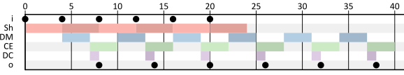
If you entered the model correctly, the CMWB gives the following
Gantt chart:
The CMWB gives the following Gantt chart:
Given the input sequence and the duration of the Sh actor, the
decoder cannot decode symbols faster than 1 symbol per 4 time units.
With two tokens on the channel from CE to DM, it operates at this
maximum rate; with only one token, it does not. So the most recent
channel-estimation information that DM can use is two symbols
old.
Exercise
2 (A producer-consumer pipeline –
creating dataflow models).
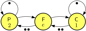
The pipeline can be modeled as follows, where \(e\in{}\{1,3\}\) is the execution time of
the filtering actor F.
With \(e=1\), the CMWB gives the
following Gantt chart:
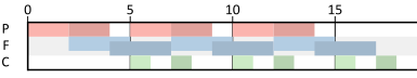
The CMWB gives the following Gantt chart when \(e=3\):
Note the overlap between firings of Actor F and the hick-ups in the
production of samples due to a full buffer between P and F.
Exercise
3 (An image-based control system –
understanding and creating dataflow models).
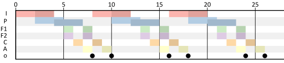
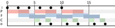
The CMWB gives the following Gantt chart:
The IBC pipeline shows a repetitive pattern in which two outputs
occur every eight time units. Hence, the average actuation rate is one
actuation per four time units. (Note that the actuation pattern is not
strictly periodic, which may be undesirable from a quality-of-control
perspective.)
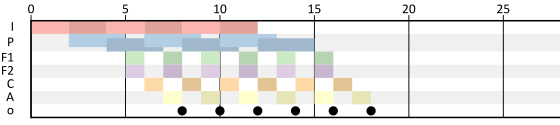
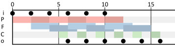
With a pipelining depth of four, the IBC pipeline operates at its
maximum actuation rate of one actuation every two time units. The
following Gantt chart can be obtained from the CMWB.
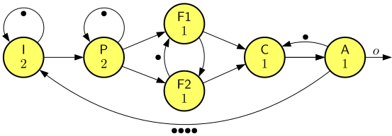
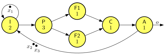
The fact that an actor is executing on a single processor can be
captured in a dataflow model with a self-loop with one initial token.
This prohibits actor executions to overlap. The mapping and scheduling
of the two feature processing actors F1 and F2 can be modeled with two
channels between those actors, one in each direction, with an initial
token on the channel to F1. The latter ensures that F1 goes first among
the two.
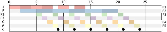
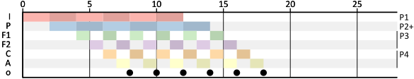
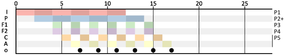
The following Gantt chart can be obtained from the CMWB. The
processors P1 to P5 that execute the actors have been added at the right
side.
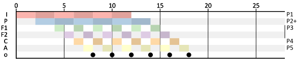
From the previous part, it is clear that the execution of Actor P
is a bottleneck. Processor P2 executing P should be sped up by at least
a factor 1.5 so that a P firing does not take more than two time units.
The following Gantt chart illustrates the execution with the improved
processor.
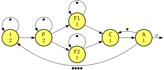
Actors C and A can be mapped onto a single processor, scheduling
their firings alternatingly, starting with C. This reduces the number of
processors to four. The dataflow model then becomes as follows:
Note that the self-loops on C and A can be omitted. The Gantt chart
does not change, except for the mapping onto processors.
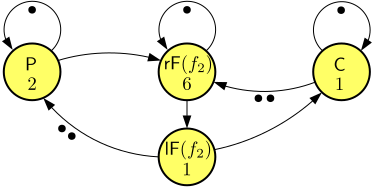
The actuation delay of the IBCS of the previous item is 8. One
option to improve it is to use faster processors. Another option is to
give both feature processing actors their own processor:
This leads to an actuation delay of 7:
Exercise
4 (A video decoder - multi-rate
dataflow).
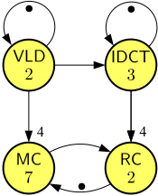
The Gantt chart shows two iterations of the following dataflow
graph.
It has a repetition vector \(\rho{}\) with \(\rho{}(VLD)=\rho{}(IDCT)=4\) and \(\rho{}(MC)=\rho{}(RC)=1\).
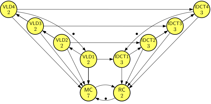
Conversion of the multi-rate dataflow model to a single-rate
dataflow graph gives the following result:
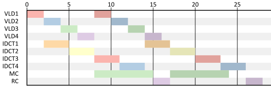
Entering this model in the CMWB gives the following Gantt
chart.
When carefully considering the firings of the four VLD and IDCT
actors, one may notice the similarity between the original Gantt chart
and this one.
Exercise
5 (An image-based control system –
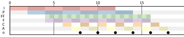
multi-rate dataflow).
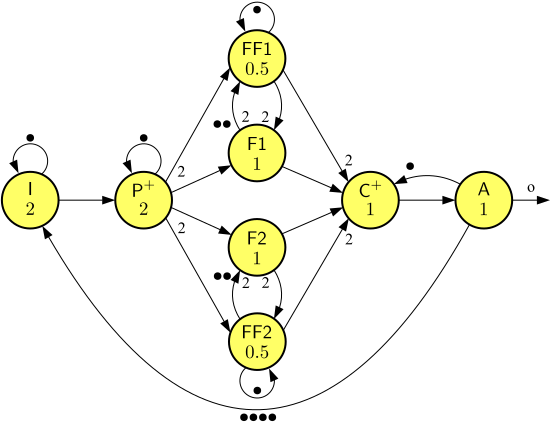
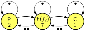
Actors I, P\(^+\), C\(^+\), and A all have an entry 1 in the
repetition vector, F has entry 2, and FF has entry 4.
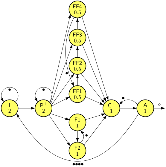
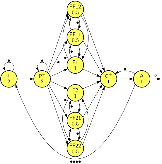
Actors I, P\(^+\), F1, F2,
C\(^+\), and A all have entry 1 in the
repetition vector, and actors FF1 and FF2 have entry 2.
Note that all four models have an actuation rate of 1 actuation per 2
time units and an actuation delay of 8.
Exercise
6 (A wireless channel decoder –
schedules, performance).
The ending of the last actor firing of a schedule determines
makespan. In both cases, this is the channel estimation actor CE. The
makespan is 40 resp. 30 for \(n=1\) and
\(n=2\).
The latency is the maximal time between the consumption of an
input token from the designated input and the production of the
corresponding output token on the designated output. For \(n=2\), this duration is constant for all
input-output token pairs, namely 8. Hence, the latency is 8. For \(n=1\), this duration grows over time,
because the DM-CE actor combination cannot keep up with the input rate.
For six iterations, the maximal duration is 18. Hence, for \(n=1\), the latency is 18.
For \(n=2\), the schedule is
periodic, because it satisfies the condition mentioned in Definition
2 (Schedules) with period \(\mu=4\); for \(n=1\), the schedule is not periodic. The
shift actor Sh fires at a higher rate than the other actors, so there is
no period \(\mu\) that can satisfy the
condition of Definition 2.
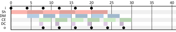
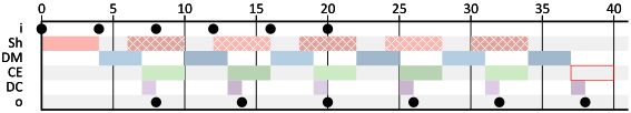
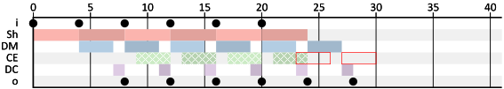
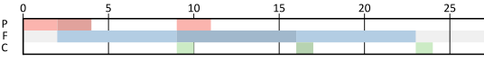
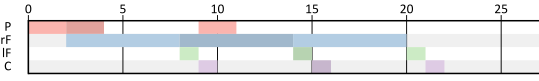
The following Gantt charts provide alap schedules for \(n=1\) and \(n=2\), respectively.
Patterned boxes are actor firings that are delayed with respect to
the self-timed schedule. Red-lined boxes illustrate actor firings that
are not needed to produce the required output, and should hence be
omitted from the schedules. Both schedules are periodic, with periods
\(\mu=6\) and \(\mu=4\), respectively.
For \(n=1\), the throughput is
\(\frac{1}{6}\); for \(n=2\), the throughput is \(\frac{1}{4}\). Note that the latency
between inputs on \(i\) and outputs on
\(o\) grows indefinitely for \(n=1\). Formally, the latency is then not
defined; informally, one might say that the latency is
infinite.
Exercise
7 (A producer-consumer pipeline –
schedules, performance).
We obtain the following Gantt chart for the first six iterations:
Assume inputs arrive periodically with period 2 and the first input
arrives at time 0.
The Gantt chart shows that the makespan is 18.
The latency grows over time. The maximum value in the schedule
for six iterations is 8.
No it isn’t. None of the actors fires in a periodic
pattern.
The above self-timed schedule is also an alap schedule for the
resulting output production.
Actor C fires 2 times per 5 time units, so the throughput is
\(\frac{2}{5}\).
The maximal achievable throughput for Actor C if the buffer
capacities may be enlarged is \(\frac{1}{2}\). The buffer between P and F
needs to be enlarged to size 3; the buffer size between F and C cannot
be decreased. We need three spaces in the P-F buffer, because each P
firing claims a space at its start and each F firing only releases a
space at its end. The following is a corresponding Gantt chart:
The self-timed schedule that maximizes throughput for the minimal
buffer capacities of the previous item is periodic with period \(\mu=2\).
The self-timed schedule is an alap schedule.
Exercise
8 (An image-based control system –
schedules, performance).
The following is a Gantt chart for the first six iterations:
The makespan is 18.
The latency is 8. Note that the latency corresponds to the actuation
delay in this example.
Yes it is. In multi-rate graphs actor firings \(k\) and \(k+\rho{}(a)\), where \(\rho{}(a)\) is the repetition-vector entry
for actor \(a\), should be at a
distance that is equal to the period. In this case, each iteration
repeats with period 2.
The self-timed schedule given above is an alap schedule.
The throughput of Actor A is \(\frac{1}{2}\). Throughput corresponds in
this example to the actuation rate.
Exercise
9 (A wireless channel decoder – max-plus
analysis).
Let \(x_{sh}(k)\), for \(k\in{}\mathbb{N}\), denote the availability
time of token \(k\) on the self-loop on
Actor Sh. By assumption \(x_{sh}(0)=0\). Let \(x_{sd}(k)\) and \(x_{dd}(k)\) be the token availability times
on the Sh-DM and DM-DC channels, respectively.
We start with expressions for the four tokens produced by the three
individual actor firings: \(x_o(k)=1\otimes
x_{dd}(k)\); \(x_{dd}(k)=3\otimes(x_{ce}(k)\oplus
x_{sd}(k))\); \(x_{sd}(k)=x_{sh}(k+1)=4\otimes(x_i(k)\oplus
x_{sh}(k))\). Note that these expressions are valid for any \(k\in{}\mathbb{N}\). Substitution yields
\(x_o(k)=1\otimes 3\otimes(x_{ce}(k)\oplus
x_{sd}(k))=4\otimes(x_{ce}(k)\oplus 4\otimes(x_i(k)\oplus
x_{sh}(k)))\). For \(k=0\), this
yields \(x_{o}(0)=4\otimes(x_{ce}(0)\oplus
4\otimes(x_i(0)\oplus x_{sh}(0)))\). Given the assumptions that
\(x_{sh}(0)=0\) and that arrival times
of tokens on inputs are non-negative, this reduces to \(x_{o}(0)=4\otimes(x_{ce}(0)\oplus 4\otimes
x_i(0))\). In the usual notations, this is equal to \(x_{o}(0)=4+\max(x_{ce}(0), 4+ x_i(0))\).
Taking as an example \(x_i(0)=x_{ce}(0)=0\) gives \(x_o(0)=8\). Note that these assumptions on
the inputs and the resulting output time conform to the Gantt chart
obtained for the first item of Exercise
1.
From the previous item, we know that \(x_{o}(1)=4\otimes(x_{ce}(1)\oplus
4\otimes(x_i(1)\oplus x_{sh}(1)))\). Substitution in combination
with the assumptions yields \(x_{o}(1)=4\otimes(x_{ce}(1)\oplus
4\otimes(x_i(1)\oplus 4\otimes(x_i(0)\oplus
x_{sh}(0))))=4\otimes(x_{ce}(1)\oplus 4\otimes(x_i(1)\oplus
4))\). In the usual notations, this leads to \(x_{o}(1)=4+\max(x_{ce}(1),4+\max(x_i(1),4))\).
Taking, in line with the Gantt chart of the first item of Exercise
1, \(x_{i}(1)=4\) and \(x_{ce}(1)=10\) leads to \(x_o(1)=4+10=14\). Also this result is in
line with the Gantt chart.
If \(x_{ce}(k)\le x_{i}(k)+4\), for
any \(k\in{}\mathbb{N}\), the
production times \(x_o(k)\) do not
depend on the arrival times \(x_{ce}(k)\), because \(x_{ce}(k)\) can be eliminated from the
expression for \(x_o(k)\) obtained in
the first item.
Exercise
10 (A wireless channel decoder –
max-plus-linear index-invariant system).
Additivity: Let \(i_1\), \(i_2\), \(ce_1\), \(ce_2\), \(o_1\), \(o_2\), and \(o_3\) be event sequences (with obvious
correspondences to inputs and outputs) such that \(i_1,ce_1\mathbin{\xrightarrow{\mathit{WCD}}}o_1\),
\(i_2,ce_2\mathbin{\xrightarrow{\mathit{WCD}}}o_2\),
and \(i_1\oplus i_2,ce_1\oplus
ce_2\mathbin{\xrightarrow{\mathit{WCD}}}o_3\). We need to show
that \(o_3=o_1\oplus o_2\).
From the previous exercise, we conclude that \(o(k)=4\otimes(ce(k)\oplus 4\otimes(i(k)\oplus
(4\otimes i)^1(k)))\) for any event sequences \(i,ce,o\) such that \(i,ce\mathbin{\xrightarrow{\mathit{WCD}}}o\).
Thus, \(o_3(k)=4\otimes((ce_1\oplus
ce_2)(k)\oplus 4\otimes((i_1\oplus i_2)(k)\oplus (4\otimes(i_1\oplus
i_2))^1(k)))\). We distinguish two cases, namely \(k=0\) and \(k>0\), because for these two cases the
delay expression \((4\otimes(i_1\oplus
i_2))^1(k)\) gives different results.
First, assume \(k=0\). Then \[\begin{array}{lcl}
o_3(0) &=& 4\otimes((ce_1\oplus ce_2)(0)\oplus
4\otimes((i_1\oplus i_2)(0)\oplus 4\otimes-\infty{})) \\
&=& 4\otimes((ce_1\oplus ce_2)(0)\oplus
4\otimes((i_1\oplus i_2)(0))) \\
&=& 4\otimes(ce_1(0)\oplus ce_2(0)\oplus 4\otimes
i_1(0)\oplus 4\otimes i_2(0)) \\
&=& 4\otimes ce_1(0)\oplus 4\otimes ce_2(0)\oplus
8\otimes i_1(0)\oplus 8\otimes i_2(0)) \\
&=& 4\otimes ce_1(0)\oplus 8\otimes i_1(0)\oplus
4\otimes ce_2(0)\oplus 8\otimes i_2(0)) \\
&=& \{\mbox{reversing the reasoning}\} \\
& & 4\otimes(ce_1(0)\oplus 4\otimes(i_1(0)\oplus
4\otimes-\infty{})) \\
& & {}\oplus 4\otimes(ce_2(0)\oplus
4\otimes(i_2(0)\oplus 4\otimes-\infty{})) \\
&=& o_1(0)\oplus o_2(0)
\end{array}
\] Note that the ‘trick’ in the above reasoning is to rewrite
\(o_3(0)\) into a sum of products.
Second, assume \(k>0\). Then
\[\begin{array}{lcl}
o_3(k) &=& 4\otimes((ce_1\oplus ce_2)(k)\oplus
4\otimes((i_1\oplus i_2)(k)\oplus(4\otimes(i_1\oplus i_2))(k-1))) \\
&=& \{\mbox{rewrite into a sum of products, similar
to the case }k=0\} \\
& & 4\otimes ce_1(k)\oplus 8\otimes i_1(k)\oplus
12\otimes i_1(k-1)\\
& & {}\oplus 4\otimes ce_2(k)\oplus 8\otimes
i_2(k)\oplus 12\otimes i_2(k-1)) \\
&=& \{\mbox{reversing the reasoning}\} \\
& & o_1(k)\oplus o_2(k)
\end{array}
\] This completes the proof of additivity.
Homogeneity: For any event sequences \(i,ce,o\) such that \(i,ce\mathbin{\xrightarrow{\mathit{WCD}}}o\)
and constant \(c\in{}\mathbb{T}\), we
need to show that \(c\otimes i,c\otimes
ce\mathbin{\xrightarrow{\mathit{WCD}}}c\otimes o\).
We start again from the earlier derived expression for \(o(k)\): \(o(k)=4\otimes(ce(k)\oplus 4\otimes(i(k)\oplus
(4\otimes i)^1(k)))\). We instantiate it with \(c\otimes i\) and \(c\otimes ce\), and again distinguish cases
\(k=0\) and \(k>0\). Assume applying WCD to \(c\otimes i\) and \(c\otimes ce\) yields output sequence \(o'\); that is, \(c\otimes i,c\otimes
ce\mathbin{\xrightarrow{\mathit{WCD}}}o'\).
First, assume \(k=0\). Then \[\begin{array}{lcl}
o'(0) &=& 4\otimes((c\otimes ce)(0)\oplus
4\otimes((c\otimes i)(0)\oplus 4\otimes-\infty{})) \\
&=& (4\otimes c\otimes ce)(0)\oplus(8\otimes c\otimes
i)(0) \\
&=& c\otimes((4\otimes ce)(0)\oplus(8\otimes i)(0)) \\
&=& c\otimes(4\otimes(ce(0)\oplus 4\otimes i(0))) \\
&=& c\otimes(4\otimes(ce(0)\oplus 4\otimes(i(0)\oplus
4\otimes-\infty{}))) \\
&=& c\otimes o(0)
\end{array}
\] The trick here is to rewrite the expression into a sum of
products, then work the multiplication with \(c\) to the outermost level, and then
reverse the reasoning.
Second, assume \(k>0\). Then,
following a similar reasoning as for case \(k=0\), it follows that \[\begin{array}{lcl}
o'(k) &=& 4\otimes((c\otimes ce)(k)\oplus
4\otimes((c\otimes i)(k)\oplus(4\otimes(c\otimes i))(k-1))) \\
&=& (4\otimes c\otimes ce)(k)\oplus(8\otimes c\otimes
i)(k)\oplus(12\otimes c\otimes i)(k-1) \\
&=& c\otimes((4\otimes ce)(k)\oplus(8\otimes
i)(k)\oplus(12\otimes i)(k-1)) \\
&=& c\otimes(4\otimes(ce(k)\oplus 4\otimes i(k)\oplus
8\otimes i(k-1))) \\
&=& c\otimes(4\otimes(ce(k)\oplus
4\otimes(i(k)\oplus(4\otimes i)(k-1)))) \\
&=& c\otimes o(k)
\end{array}
\] This proves homogeneity.
Index invariance: For any event sequences \(i,ce,o\) such that \(i,ce\mathbin{\xrightarrow{\mathit{WCD}}}o\)
and \(N\in{}\mathbb{N}\), we need to
show that \({{i}^{N}},{{ce}^{N}}\mathbin{\xrightarrow{\mathit{WCD}}}{{o}^{N}}\).
Assume \({{i}^{N}},{{ce}^{N}}\mathbin{\xrightarrow{\mathit{WCD}}}o'\).
We start from \(o'(k)=4\otimes({{ce}^{N}}(k)\oplus
4\otimes({{i}^{N}}(k)\oplus (4\otimes {{i}^{N}})^1(k)))\). We
distinguish cases \(N=0\), \(k<N\), \(0<k=N\), and \(k>N\).
For \(N=0\), the result follows
immediately because \({{s}^{0}}=s\) for
any event sequence \(s\).
For \(k<N\), it follows easily
that \(o'(k)=-\infty{}={{o}^{N}}(k)\).
Exercise
11 (The manufacturing system
– superposition).
The CMWB can be used to generate the needed output event sequences
for all input event sequences of interest. The CMWB can also be used to
check the correctness of the outcomes derived through superposition.
The production times are then as follows:
[16,21,26,33,40].
The production times are then as follows:
[16,21,28,33,38].
The production times can be obtained by taking the element-wise
maximum of the results of the previous items: [16,21,28,33,40].
The output production times resulting from an input sequence
[5,\(-\infty{}\),\(-\infty{}\),\(-\infty{}\),\(-\infty{}\)] are [16,22,27,32,37]. Hence,
compared to the production times obtained earlier, the second output
will be delayed by 1 time unit.
The output production times resulting from input sequence [4,\(-\infty{}\),\(-\infty{}\),\(-\infty{}\),\(-\infty{}\)] are [16,21,26,31,36]. So the
best possible makespan with the first bottom arriving at time 4 is equal
to 36. This makespan cannot be further improved. Assuming the unlimited
availability of bottoms and tops at time 0 gives the same makespan. (It
in fact gives exactly the same production times for all outputs.)
The response to input sequence [5,\(-\infty{}\),\(-\infty{}\),\(-\infty{}\),\(-\infty{}\)] shows that the arrival of the
first bottom cannot be further delayed than time 4 without affecting the
best possible makespan. The makespan of any schedule in which the first
bottom arrives at time 5 cannot be better than 37.
Exercise
12 (A wireless channel decoder – impulse
responses).
We need to constrain only the first firing; all other firings
automatically get starting times at least 0 because of the dependencies.
Therefore, \(sh=[0, -\infty{},
-\infty{},-\infty{},\ldots]=\delta{}\) is sufficient. \(sh=[0, 0, 0, \ldots]\) is also possible and
leads to the same result, but the following analysis would be more
involved.
\(h_{i,o}=[8,\)\(12,\)\(16,\)\(20,\)\(24,\ldots]\), \(h_{ce,o}=[4,-\infty{},-\infty{},-\infty{},-\infty{},\ldots]\),
and \(h_{sh,o}=[8,\)\(12,\)\(16,\)\(20,\)\(24,\ldots]\).
Using the generalization of Theorem 4
to systems with multiple inputs and outputs, we obtain \(o=i\otimes h_{i,o}\oplus ce\otimes h_{ce,o}\oplus
sh \otimes h_{sh,o}=i\otimes h_{i,o}\oplus ce\otimes
h_{ce,o}\oplus\delta\otimes h_{sh,o}\).
Assuming \({\textrm{\bf{}{G}}}\)
denotes the above matrix, we can compute the makespan of the first
iteration as \(\left|{{\textrm{\bf{}{x}}}(1)}\right|=\left|{{\textrm{\bf{}{G}}}{\bf{0}}}\right|=\left|{[2~0~5~0~6~6]^T}\right|=6\).
The makespan of the second iteration is \(\left|{{\textrm{\bf{}{x}}}(2)}\right|=\left|{{\textrm{\bf{}{G}}}{\textrm{\bf{}{x}}}(1)}\right|=\left|{[4~5~7~6~8~8]^T}\right|=8\).
Finally, the makespan of the third iteration then is \(\left|{{\textrm{\bf{}{G}}}{\textrm{\bf{}{x}}}(2)}\right|=\left|{[7~7~10~8~11~11]^T}\right|=11\).
Exercise
14 (A producer-consumer
pipeline – symbolic simulation).
The symbolic simulation can only be performed in one order, starting
with P, followed by F, and ending with C:
The symbolic time-stamp vector for \(x_1\) is the completion time of P; the
symbolic time-stamp vector for \(x_2\)
is the initial time-stamp vector for \(x_3\), \({{\textrm{\bf{}{i}}}_{3}}\); for \(x_3\), we take the completion time of F,
for \(x_4\), the initial time-stamp
vector for \(x_5\), \({{\textrm{\bf{}{i}}}_{5}}\), and for \(x_5\) and \(x_6\), the completion time of C. The end
result is, not surprisingly, the same matrix \({\textrm{\bf{}{G}}}\) as in the previous
exercise.
Exercise
15 (An image-based control
pipeline – symbolic simulation).
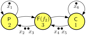
We name the time stamps as in the following picture:
The symbolic simulation goes as follows:
actor
symbolic start
symbolic completion
I
\([ ~ 0 ~ 0 ~
-\infty{} ]^{T}\)
\([ ~ 2 ~ 2 ~
-\infty{} ]^{T}\)
P
\([ ~ 2 ~ 2 ~
-\infty{} ]^{T}\)
\([ ~ 5 ~ 5 ~
-\infty{} ]^{T}\)
F1
\([ ~ 5 ~ 5 ~
-\infty{} ]^{T}\)
\([ ~ 6 ~ 6 ~
-\infty{} ]^{T}\)
F2
\([ ~ 5 ~ 5 ~
-\infty{} ]^{T}\)
\([ ~ 6 ~ 6 ~
-\infty{} ]^{T}\)
C
\([ ~ 6 ~ 6 ~
-\infty{} ]^{T}\)
\([ ~ 7 ~ 7 ~
-\infty{} ]^{T}\)
A
\([ ~ 7 ~ 7 ~
-\infty{} ]^{T}\)
\([ ~ 8 ~ 8 ~
-\infty{} ]^{T}\)
The symbolic time-stamp vector for \(x_1\) is the completion time of I; the
symbolic time-stamp vector for \(x_2\)
is the initial time-stamp vector for \(x_3\), \({{\textrm{\bf{}{i}}}_{3}}\); for \(x_3\), we get the completion time of A.
This gives matrix \[ {\textrm{\bf{}{G}}}=
\begin{bmatrix}
2 & 2 & -\infty{} \\
-\infty{} & -\infty{} & 0 \\
8 & 8 & -\infty{}
\end{bmatrix}
\]
To compute the makespan of the first three actuations, we compute
\(\left|{{\textrm{\bf{}{G}}}^3{\bf{0}}}\right|\).
The series of time-stamp vectors obtained during the computation is
\([2~0~8]^T\), \([4~8~10]^T\), \([10~10~16]^T\). The norm of the last
vector, and therefore the makespan of three actuations, is 16. As a next
step, we compute \({\textrm{\bf{}{G}}}^4{\bf{0}}={\textrm{\bf{}{G}}}[10~10~16]^T=[12~16~18]^T\).
The fifth sample period starts when both the tokens (corresponding to)
\(x_1\) and \(x_2\) have been reproduced after four
iterations. That is, the fifth sample period starts at \(12\oplus 16=16\). You may check that these
results conform to the Gantt chart for this IBC pipeline in Exercise
3.
Exercise
16 (A producer-consumer pipeline – worst-case
abstractions).
The worst-case response time of Actor F is 7, when the pipeline
gets two consecutive time slots in the TDM schedule and the data arrives
precisely at the end of its turn in the TDM schedule. This can be
captured in the model as follows. Note the self-edge that captures the
fact that different executions of F cannot overlap when executing on the
same processor.
Under the mentioned TDM scheduling, Actor F gets 50% of the
processing time and has a workload of 3. So the average rate is \(1/6\). A worst-case latency of 1 needs to
be added to be conservative. Note that F is guaranteed to have 3 time
slots in any consecutive 7 time slots in the schedule, so it always
completes within 7 time units. This can be modeled as follows.
The real worst-case conditions occur when the first data arrives
for Actor F to process, but its turn in the TDM schedule has just
passed. We then get the following Gantt chart, where patterned boxes
show that the processing of F has been suspended. The makespan of the
third iteration is 22.
The model with the worst-case response time of F as the actor
execution time gives the following Gantt chart. The makespan of the
third iteration according to this model is 24.
The Gantt chart for the model with a latency-rate model for F is as
follows, with a makespan of 22 for three iterations.
Observe that indeed the two models of the first two items are
conservative, but they are also both pessimistic. The last model
accurately predicts the makespan of (one and) three iterations, but it
is pessimistic for the second iteration.
Exercise
17 (An image-based control system –
eigenvalue, eigenvector).
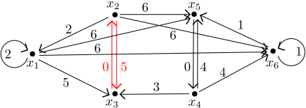
We obtain the following precedence graph from the matrix computed
in Exercise 15.
The MCM is \(\frac{8}{2}=4\),
derived from the cycle in red. So the eigenvalue is 4.
We obtain the following precedence graph for the eigenvector by
subtracting the eigenvalue 4 from each of the edge weights.
We now select node \(x_2\) on the
critical cycle. The longest paths to nodes \(x_1\), \(x_2\), and \(x_3\) are then \(-2\), \(0\), and \(4\), respectively. This gives normal
eigenvector \([{-6}~{-4}~0]^T\).
With initial-token time stamps \([0~2~6]^T\), we obtain the following
periodic schedule. \[
\left\{
\begin{array}{l}
\sigma{}(I, k) = 2 + 4k\\
\sigma{}(P, k) = 4 + 4k\\
\sigma{}(F1, k) = \sigma{}(F2, k) = 7 + 4k\\
\sigma{}(C, k) = 8 + 4k\\
\sigma{}(A, k) = 9 + 4k
\end{array}
\right.
\]
Exercise
18 (A producer-consumer pipeline –
eigenvalue, eigenvector).
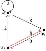
We obtain the following precedence graph from the matrix computed
in Exercise 13.
The MCM is \(\frac{5}{2}=2.5\),
derived from the cycle in red. So the eigenvalue is \(2.5\). The critical cycle corresponds to
the P–F cycle in the dataflow graph.
We may obtain a precedence graph for the eigenvector by
subtracting the eigenvalue 2.5 from each of the edge weights. Selecting
node \(x_2\) on the critical cycle
gives eigenvector \([{-0.5}~{0}~{2.5}~{1}~{3.5}~{3.5}]^T\).
Normalizing this vector gives \([{-4}~{-3.5}~{-1}~{-2.5}~{0}~{0}]^T\).
With initial-token time stamps \([{0}~{0.5}~{3}~{1.5}~{4}~{4}]^T\), we
obtain the following periodic schedule. \[
\left\{
\begin{array}{l}
\sigma{}(P, k) = 0.5 + 2.5k\\
\sigma{}(F, k) = 2.5 + 2.5k\\
\sigma{}(C, k) = 5.5 + 2.5k
\end{array}
\right.
\]
Exercise
19 (A wireless channel decoder –
state-space model).
We collect state and input vectors into a single vector as
follows: \([\,{\textrm{\bf{}{x}}}^T~i~ce\,]^T\) with
\({\textrm{\bf{}{x}}}=[\,x_1~x_2~x_3~x_4\,]^T\).
The symbolic simulation goes as follows:
The symbolic time-stamp vectors for \(x_1\) and \(x_2\) are the completion times of Sh and
DM; the symbolic time-stamp vector for \(x_3\) is the initial time-stamp vector for
\(x_4\); for \(x_4\), we get the completion time of CE.
For output \(o\), we get the completion
time of DC. This gives the following result: \[
\begin{bmatrix}{\textrm{\bf{}{A}}}&{\textrm{\bf{}{B}}}\\{\textrm{\bf{}{C}}}&{\textrm{\bf{}{D}}}\\\end{bmatrix}
=
\left[
\begin{array}{ccccc|ccc}
& 4 & -\infty{} & -\infty{} & -\infty{} & 4 &
-\infty{} & \\
& 7 & 3 & 3 & -\infty{} & 7 & 3 & \\
& -\infty{} & -\infty{} & -\infty{} & 0 &
-\infty{} & -\infty{} & \\
& 10 & 6 & 6 & -\infty{} & 10 & 6 & \\
& 8 & 4 & 4 & -\infty{} & 8 & 4 & \\
\end{array}
\right]
\] with \[
\left[\begin{array}{c}{{\textrm{\bf{}{x}}}(k+1)}\\{o(k)}\\\end{array}\right]
=
\begin{bmatrix}{\textrm{\bf{}{A}}}&{\textrm{\bf{}{B}}}\\{\textrm{\bf{}{C}}}&{\textrm{\bf{}{D}}}\\\end{bmatrix}
\begin{bmatrix}{{\textrm{\bf{}{x}}}(k)}\\{i(k)}\\{ce(k)}\end{bmatrix}
\]
We first take for input \(i\)
the impulse sequence \(\delta{}\). For
\(ce\), we take \(\epsilon{}\), the sequence of only \(-\infty{}\) values. For initial state \({\textrm{\bf{}{x}}}(0)\), we take \(\bf{\epsilon}\), the vector containing only
\(-\infty{}\) as its elements. Using
the max-plus representation of the dataflow model, we can then compute
the impulse response \(\overline{{\textrm{\bf{}{h}}}}_i\) up to
the first four outputs as follows: \[
\overline{{\textrm{\bf{}{h}}}}_i(0)
=
\left[\begin{array}{c}{{\textrm{\bf{}{x}}}(1)}\\{o(0)}\\\end{array}\right]
=
\begin{bmatrix}{\textrm{\bf{}{A}}}&{\textrm{\bf{}{B}}}\\{\textrm{\bf{}{C}}}&{\textrm{\bf{}{D}}}\\\end{bmatrix}\begin{bmatrix}{{\textrm{\bf{}{x}}}(0)}\\{i(0)}\\{ce(0)}\end{bmatrix}
=
\begin{bmatrix}{\textrm{\bf{}{A}}}&{\textrm{\bf{}{B}}}\\{\textrm{\bf{}{C}}}&{\textrm{\bf{}{D}}}\\\end{bmatrix}\begin{bmatrix}{\bf{\epsilon}}\\{0}\\{-\infty{}}\end{bmatrix}
= \begin{bmatrix}{4}\\{7}\\{-\infty{}}\\{10}\\{8}\end{bmatrix}
\]\[
\overline{{\textrm{\bf{}{h}}}}_i(1)
=
\left[\begin{array}{c}{{\textrm{\bf{}{x}}}(2)}\\{o(1)}\\\end{array}\right]
=
\begin{bmatrix}{\textrm{\bf{}{A}}}&{\textrm{\bf{}{B}}}\\{\textrm{\bf{}{C}}}&{\textrm{\bf{}{D}}}\\\end{bmatrix}\begin{bmatrix}{{\textrm{\bf{}{x}}}(1)}\\{i(1)}\\{ce(1)}\end{bmatrix}
=
\begin{bmatrix}{\textrm{\bf{}{A}}}&{\textrm{\bf{}{B}}}\\{\textrm{\bf{}{C}}}&{\textrm{\bf{}{D}}}\\\end{bmatrix}\begin{bmatrix}{4}\\{7}\\{-\infty{}}\\{10}\\{-\infty{}}\\{-\infty{}}\end{bmatrix}
= \begin{bmatrix}{8}\\{11}\\{10}\\{14}\\{12}\end{bmatrix}
\]\[
\overline{{\textrm{\bf{}{h}}}}_i(2)
=
\left[\begin{array}{c}{{\textrm{\bf{}{x}}}(3)}\\{o(2)}\\\end{array}\right]
=
\begin{bmatrix}{\textrm{\bf{}{A}}}&{\textrm{\bf{}{B}}}\\{\textrm{\bf{}{C}}}&{\textrm{\bf{}{D}}}\\\end{bmatrix}\begin{bmatrix}{{\textrm{\bf{}{x}}}(2)}\\{i(2)}\\{ce(2)}\end{bmatrix}
=
\begin{bmatrix}{\textrm{\bf{}{A}}}&{\textrm{\bf{}{B}}}\\{\textrm{\bf{}{C}}}&{\textrm{\bf{}{D}}}\\\end{bmatrix}\begin{bmatrix}{8}\\{11}\\{10}\\{14}\\{-\infty{}}\\{-\infty{}}\end{bmatrix}
= \begin{bmatrix}{12}\\{15}\\{14}\\{18}\\{16}\end{bmatrix}
\]\[
\overline{{\textrm{\bf{}{h}}}}_i(3)
=
\left[\begin{array}{c}{{\textrm{\bf{}{x}}}(4)}\\{o(3)}\\\end{array}\right]
=
\begin{bmatrix}{\textrm{\bf{}{A}}}&{\textrm{\bf{}{B}}}\\{\textrm{\bf{}{C}}}&{\textrm{\bf{}{D}}}\\\end{bmatrix}\begin{bmatrix}{{\textrm{\bf{}{x}}}(3)}\\{i(3)}\\{ce(3)}\end{bmatrix}
=
\begin{bmatrix}{\textrm{\bf{}{A}}}&{\textrm{\bf{}{B}}}\\{\textrm{\bf{}{C}}}&{\textrm{\bf{}{D}}}\\\end{bmatrix}\begin{bmatrix}{12}\\{15}\\{14}\\{18}\\{-\infty{}}\\{-\infty{}}\end{bmatrix}
= \begin{bmatrix}{16}\\{19}\\{18}\\{22}\\{20}\end{bmatrix}
\] It is not difficult to see that \(\overline{{\textrm{\bf{}{h}}}}_i\) proceeds
in a periodic pattern with period 4.
In a similar fashion, we can compute the impulse response \(\overline{{\textrm{\bf{}{h}}}}_{ce}\):
\[ \overline{{\textrm{\bf{}{h}}}}_{ce}(0)
=
\begin{bmatrix}{\textrm{\bf{}{A}}}&{\textrm{\bf{}{B}}}\\{\textrm{\bf{}{C}}}&{\textrm{\bf{}{D}}}\\\end{bmatrix}\begin{bmatrix}{\bf{\epsilon}}\\{-\infty{}}\\{0}\end{bmatrix}
= \begin{bmatrix}{-\infty{}}\\{3}\\{-\infty{}}\\{6}\\{4}\end{bmatrix}
,~ \overline{{\textrm{\bf{}{h}}}}_{ce}(1)
=
\begin{bmatrix}{\textrm{\bf{}{A}}}&{\textrm{\bf{}{B}}}\\{\textrm{\bf{}{C}}}&{\textrm{\bf{}{D}}}\\\end{bmatrix}\begin{bmatrix}{-\infty{}}\\{3}\\{-\infty{}}\\{6}\\{-\infty{}}\\{-\infty{}}\end{bmatrix}
= \begin{bmatrix}{-\infty{}}\\{6}\\{6}\\{9}\\{7}\end{bmatrix}
\]\[
\overline{{\textrm{\bf{}{h}}}}_{ce}(2)
=
\begin{bmatrix}{\textrm{\bf{}{A}}}&{\textrm{\bf{}{B}}}\\{\textrm{\bf{}{C}}}&{\textrm{\bf{}{D}}}\\\end{bmatrix}\begin{bmatrix}{-\infty{}}\\{6}\\{6}\\{9}\\{-\infty{}}\\{-\infty{}}\end{bmatrix}
= \begin{bmatrix}{-\infty{}}\\{9}\\{9}\\{12}\\{10}\end{bmatrix}
,~ \overline{{\textrm{\bf{}{h}}}}_{ce}(3)
=
\begin{bmatrix}{\textrm{\bf{}{A}}}&{\textrm{\bf{}{B}}}\\{\textrm{\bf{}{C}}}&{\textrm{\bf{}{D}}}\\\end{bmatrix}\begin{bmatrix}{-\infty{}}\\{9}\\{9}\\{12}\\{-\infty{}}\\{-\infty{}}\end{bmatrix}
= \begin{bmatrix}{-\infty{}}\\{12}\\{12}\\{15}\\{13}\end{bmatrix}
\] It is not difficult to see that \(\overline{{\textrm{\bf{}{h}}}}_{ce}\)
proceeds in a periodic pattern with period 3.
The assumptions imply that we can take for \(ce\) the \(\epsilon{}\) sequence and for initial state
\({\textrm{\bf{}{x}}}\) the zero vector
\({\bf{0}}\). From this we can again
compute the outputs with the state-space equations. \[ \left[\begin{array}{c}{{\textrm{\bf{}{x}}}(1)}\\{o(0)}\\\end{array}\right]
=
\begin{bmatrix}{\textrm{\bf{}{A}}}&{\textrm{\bf{}{B}}}\\{\textrm{\bf{}{C}}}&{\textrm{\bf{}{D}}}\\\end{bmatrix}\begin{bmatrix}{{\bf{0}}}\\{0}\\{-\infty{}}\end{bmatrix}
= \begin{bmatrix}{4}\\{7}\\{0}\\{10}\\{8}\end{bmatrix}
,~ \left[\begin{array}{c}{{\textrm{\bf{}{x}}}(2)}\\{o(1)}\\\end{array}\right]
=
\begin{bmatrix}{\textrm{\bf{}{A}}}&{\textrm{\bf{}{B}}}\\{\textrm{\bf{}{C}}}&{\textrm{\bf{}{D}}}\\\end{bmatrix}\begin{bmatrix}{4}\\{7}\\{0}\\{10}\\{4}\\{-\infty{}}\end{bmatrix}
= \begin{bmatrix}{8}\\{11}\\{10}\\{14}\\{12}\end{bmatrix}
\]\[ \left[\begin{array}{c}{{\textrm{\bf{}{x}}}(3)}\\{o(2)}\\\end{array}\right]
=
\begin{bmatrix}{\textrm{\bf{}{A}}}&{\textrm{\bf{}{B}}}\\{\textrm{\bf{}{C}}}&{\textrm{\bf{}{D}}}\\\end{bmatrix}\begin{bmatrix}{8}\\{11}\\{10}\\{14}\\{8}\\{-\infty{}}\end{bmatrix}
= \begin{bmatrix}{12}\\{15}\\{14}\\{18}\\{16}\end{bmatrix}
,~ \left[\begin{array}{c}{{\textrm{\bf{}{x}}}(4)}\\{o(3)}\\\end{array}\right]
=
\begin{bmatrix}{\textrm{\bf{}{A}}}&{\textrm{\bf{}{B}}}\\{\textrm{\bf{}{C}}}&{\textrm{\bf{}{D}}}\\\end{bmatrix}\begin{bmatrix}{12}\\{15}\\{14}\\{18}\\{12}\\{-\infty{}}\end{bmatrix}
= \begin{bmatrix}{16}\\{19}\\{18}\\{22}\\{20}\end{bmatrix}
\] Not surprisingly, self-timed execution follows the impulse
response for input \(i\).
The first firing of Actor CE produces token \(x_4(1)\), which is the third token on the
channel to DM. We can analyze the impact of delaying the production of
this token through the impulse response for channel \(ce\). From the previous item, we know that
\(x_4(1)=10\). So if the execution time
of the firing producing this token takes one additional time unit, then
it is produced at time 11. We can analyze the effect of this in two
steps. First, we constrain the firing of DM that needs this specific
token by delaying the impulse response \(\overline{{\textrm{\bf{}{h}}}}_{ce}\) by
two samples and a time delay of 11: \[
11\otimes{{\overline{{\textrm{\bf{}{h}}}}_{ce}}^{2}} =
\begin{bmatrix}{-\infty{}}\\{-\infty{}}\\{-\infty{}}\\{-\infty{}}\\{-\infty{}}\end{bmatrix},
\begin{bmatrix}{-\infty{}}\\{-\infty{}}\\{-\infty{}}\\{-\infty{}}\\{-\infty{}}\end{bmatrix},
\begin{bmatrix}{-\infty{}}\\{14}\\{-\infty{}}\\{17}\\{15}\end{bmatrix},
\begin{bmatrix}{-\infty{}}\\{17}\\{17}\\{20}\\{18}\end{bmatrix},
\ldots
\] Second, through superposition, we can then compute the effect
on the self-timed execution. Assume \({\bf{\sigma{}}}\) is the schedule computed
in the previous item. We then get that \[
{\bf{\sigma{}}}\oplus
11\otimes{{\overline{{\textrm{\bf{}{h}}}}_{ce}}^{2}} = {\bf{\sigma{}}}
\] Hence, the delay in the first firing of Actor CE has no effect
on the decoder output.
Exercise
20 (A wireless channel decoder –
throughput).
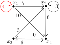
We obtain the following precedence graph from the \({\textrm{\bf{}{A}}}\) matrix computed in
Exercise 19.
The MCM is \(4\), derived from the
self-edge in red, corresponding to the self-edge of Actor Sh in the
dataflow graph. So the eigenvalue of \({\textrm{\bf{}{A}}}\) is \(\lambda{}=4\). From the \({\textrm{\bf{}{C}}}\) matrix (see Exercise
19) and the precedence graph, it
can be concluded that output \(o\)
depends on all four state-vector elements. So from Theorem
5, it follows that the maximal throughput
that the decoder may achieve is \(\frac{1}{4}\).
Exercise
21 (An image-based control system –
throughput).
In Exercise 15, we
computed matrix \({\textrm{\bf{}{G}}}\)
with symbolic simulation. Since the dataflow graph does not have any
inputs, \({\textrm{\bf{}{G}}}\) equals
the \({\textrm{\bf{}{A}}}\) matrix in
the full state-space model. Moreover, the state-space model does not
have any \({\textrm{\bf{}{B}}}\) and
\({\textrm{\bf{}{D}}}\) matrices.
Matrix \({\textrm{\bf{}{C}}}=
[~8~8~-\infty{}~]\) follows immediately from the symbolic
simulation of Exercise 15.
The eigenvalue of \({\textrm{\bf{}{A}}}\) is 4, as derived in
Exercise 17. From the \({\textrm{\bf{}{C}}}\) matrix and the
precedence graph derived in Exercise
17, it follows that Theorem
5 applies. Hence, the maximal throughput
of the IBC pipeline is \(\frac{1}{4}\).
Exercise
22 (A producer-consumer pipeline –
throughput).
To compute the state-space model of the graph, we perform
symbolic simulation.
The \({\textrm{\bf{}{A}}}\) matrix
equals the \({\textrm{\bf{}{G}}}\)
matrix derived in Exercise 13 for which the
eigenvalue, 2.5, was computed in Exercise
18. From the \({\textrm{\bf{}{C}}}\) matrix and the
precedence graph derived in Exercise 18,
it follows that Theorem 5 applies. Hence,
the maximal throughput of the producer-consumer pipeline is \(\frac{1}{2.5}=\frac{2}{5}\).
The wireless channel decoder of Exercise
20 has a throughput of \(\frac{1}{4}\). The producer-consumer
pipeline is slowed down to follow this throughput (Theorem
6). Thus the throughput of the overall
system is \(\frac{1}{4}\).
Exercise
23 (An image-based control system –
latency).
The state-space model was derived in Exercise
21. The \({\textrm{\bf{}{A}}}\) matrix is the matrix
\({\textrm{\bf{}{G}}}\) of Exercise
15, the \({\textrm{\bf{}{C}}}\) matrix is \([~8~8~-\infty{}~]\). Since the graph has no
inputs, the model does not have \({\textrm{\bf{}{B}}}\) and \({\textrm{\bf{}{D}}}\) matrices. To compute
the desired latency, we only need to compute \({\bf{}\Lambda}_{\mathit{state}}^{\mu{}}\)
for \(\mu{}=4\): \[
-\mu{}\otimes{\textrm{\bf{}{A}}}=
-4\otimes\begin{bmatrix}
2 & 2 & -\infty{} \\
-\infty{} & -\infty{} & 0 \\
8 & 8 & -\infty{}
\end{bmatrix}
=
\begin{bmatrix}
-2 & -2 & -\infty{} \\
-\infty{} & -\infty{} & -4 \\
4 & 4 & -\infty{}
\end{bmatrix}
\]
Exercise
24 (A wireless channel decoder –
latency).
Recall the state-space model of Exercise
19. We compute the two latency
matrices as follows, using the CMWB to compute the \(*\)-closure: \[
-4\otimes{\textrm{\bf{}{A}}} =
\begin{bmatrix}
0 & -\infty{} & -\infty{} & -\infty{} \\
3 & -1 & -1 & -\infty{} \\
-\infty{} & -\infty{} & -\infty{} & -4 \\
6 & 2 & 2 & -\infty{} \\
\end{bmatrix}
\]\[
(-\mu{}\otimes{}{\textrm{\bf{}{A}}})^*=
\begin{bmatrix}
0 & -\infty{} & -\infty{} & -\infty{} \\
3 & 0 & -1 & -5 \\
2 & -2 & 0 & -4 \\
6 & 2 & 2 & 0 \\
\end{bmatrix}
\]\[
{\bf{}\Lambda}_{\mathit{state}}^{\mu{}} =
{\textrm{\bf{}{C}}}\left({-\mu{}}\otimes{}{\textrm{\bf{}{A}}}
\right)^{*}
= \begin{bmatrix}{8}~{4}~{4}~{-\infty{}}\end{bmatrix}
\begin{bmatrix}
0 & -\infty{} & -\infty{} & -\infty{} \\
3 & 0 & -1 & -5 \\
2 & -2 & 0 & -4 \\
6 & 2 & 2 & 0 \\
\end{bmatrix}
= \begin{bmatrix}{8}~{4}~{4}~{0}\end{bmatrix}
\]\[
{\bf{}\Lambda}_{\mathit{IO}}^{\mu{}} =
{\bf{}\Lambda}_{\mathit{state}}^{\mu{}} \left(
-\mu{}\otimes{}{\textrm{\bf{}{B}}} \right) \oplus {\textrm{\bf{}{D}}}
= \begin{bmatrix}{8}~{4}~{4}~{0}\end{bmatrix}
\begin{bmatrix}
0 & -\infty{} \\
3 & -1 \\
-\infty{} & -\infty{} \\
6 & 2 \\
\end{bmatrix}
\oplus\begin{bmatrix}{8}~{4}\end{bmatrix}
= \begin{bmatrix}{8}~{3}\end{bmatrix}
\oplus\begin{bmatrix}{8}~{4}\end{bmatrix} =
\begin{bmatrix}{8}~{4}\end{bmatrix}
\] Because the inputs are assumed to be the 4-periodic event
sequence, their latency is 0. Since the initial tokens are available at
time 0, we can compute the desired latency therefore as follows: \[
L(o,4)=\begin{bmatrix}{8}~{4}~{4}~{0}\end{bmatrix}{\bf{0}}\oplus\begin{bmatrix}{8}~{4}\end{bmatrix}{\bf{0}}=8
\]
Exercise
25 (A producer-consumer pipeline –
latency).
Using the CMWB, we obtain the state-latency and IO-latency matrices:
\[
{\bf{}\Lambda}_{\mathit{state}}^{\mu{}}=\begin{bmatrix}{6}~{6}~{3.5}~{1}~{4}~{1.5}\end{bmatrix},
{\bf{}\Lambda}_{\mathit{IO}}^{\mu{}} =
\left[\begin{array}{c}{6}\\\end{array}\right]
\] So \[
L(o,2.5)=\begin{bmatrix}{6}~{6}~{3.5}~{1}~{4}~{1.5}\end{bmatrix}{\bf{0}}\oplus\left[\begin{array}{c}{6}\\\end{array}\right]{\bf{0}}=6
\]
We know from Exercise 24 that the
latency of the channel decoder is \(L(o,4)=8\). We can recompute the latency of
our producer-consumer pipeline for a period of \(\mu{}=4\) as \[
{\bf{}\Lambda}_{\mathit{state}}^{\mu{}}=\begin{bmatrix}{6}~{6}~{2}~{1}~{4}~{0}\end{bmatrix},
{\bf{}\Lambda}_{\mathit{IO}}^{\mu{}} =
\left[\begin{array}{c}{6}\\\end{array}\right]
\] Assuming a latency of 8 for its input from the channel decoder
we get: \[
L(o,4)=\begin{bmatrix}{6}~{6}~{2}~{1}~{4}~{0}\end{bmatrix}{\bf{0}}\oplus\left[\begin{array}{c}{6}\\\end{array}\right]\left[\begin{array}{c}{8}\\\end{array}\right]=14
\] Thus, the combined system has a latency of 14. (Note that, in
this case, the latency of the combined system is the sum of the
latencies of the two constituent systems. This is not in general true.
You may try to construct an example.)
Exercise
26 (A wireless channel decoder –
stability).
No, this self-timed schedule is not stable. The self-timed
schedule produces an output \(o(k)\) at
times \(8+4k\), for all \(k\). We can consider a simple disturbance
of a delay of 1 on the initial input on \(i\). That is, we assume input \(1\otimes\delta{}\) for \(i\) and determine its effect on the
self-timed schedule through superposition. In Exercise
19, we computed the impulse
response \(\overline{{\textrm{\bf{}{h}}}}_i\). From
this, we know that \(o(k)\) occurs at
times \(8+4k\) in this impulse
response. So when delaying the impulse input with 1 time unit, to \(1\otimes\delta{}\), \(o(k)\) occurs at times \(9+4k\). Through superposition with
production times \(8+4k\), we know that
\(o(k)\) also occurs at times \(9+4k\) in the self-timed schedule with a
delayed first input. Hence, all outputs are delayed by 1 time unit,
showing instability.
Yes, the schedule is stable. From the impulse response \(\overline{{\textrm{\bf{}{h}}}}_{ce}\)
computed in Exercise 19 (which is
also valid for the adapted model; why?), we know that \(o(k)\) occurs at times \(4+3k\) in this impulse response. So if we
delay any input \(m\) of the \(ce\) input by an arbitrary constant \(c\), then we know that \(o(k)\) for \(k\ge
m\) occurs at \(4+c+3k\) in the
delayed impulse response. Through superposition, and since \(4+c+3k\le 4+4k\) for any \(k\ge m+c\), it follows that the disturbance
dissolves in the self-timed schedule after (at most) \(c\) outputs. Hence, the self-timed schedule
is stable. (Observe that this example illustrates that a schedule may be
stable even if it requires the maximal sustainable throughput. The
reason is that the actor that limits the throughput does not depend on
the input.)