Example 15 (Variable Response Times)

Assume that we want to model tasks executing on a processor that employs round-robin arbitration between three applications. The arbitration works as follows. It offers service of the processor to the three applications in a cyclic fashion. When the application has workload to perform, it can use the processor until all its work is done, or until it has used the processor for the maximum period \(P\), whichever comes first. After that, or immediately, in case the application did not have any work to perform, the arbitration turns to the following application in the cycle and offers service to that application. This process continues. When none of the applications has any workload, the processor idles until one of the applications has some workload again.

From the perspective of one of the applications, the system is not deterministic. The behavior may vary with the workload of other applications. Assume the period of the round-robin arbitration is \(P=4\) and the application needs to execute tasks which need the processor for \(10\) time units. Then, in the best case, it takes exactly \(10\) time units to complete if the other applications do not require the processor service. In the worst case, it may take \(34\) time units. The processor may be allocated to both other applications first for two periods (8 time units) Then the 10 time units are interrupted twice, after 4 and again after 8 time units with two more interruptions of two periods each. Any duration in between \(10\) and \(34\) is also possible.

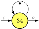
This means we could model the task execution with the following dataflow model.

Note that the self-edge prevents multiple instances of the task from executing simultaneously, which is not possible as they would need the same processor. Hence, a deterministic worst-case model exists of the processor which is itself not deterministic. Monotonicity of the dataflow model ensures that any performance metrics we derive using the dataflow model are conservative with respect to the actual performance with the real round-robin arbitration.

The simple model we derived above is, however, more pessimistic than necessary. Imagine for example that two task instances arrive together. They need a total of 20 time units of the processor. With similar reasoning as applied above, we can conclude that this requires in the worst case, 60 time units, but the dataflow model above predicts 68 time units.

The reason is that the worst-case conditions that determine the response time of 34 for a single task cannot occur also for the second task if the processing of the second task immediately follows the processing of the first.

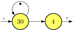
We often use the following type of dataflow model instead, which is more accurate. It is called a latency-rate dataflow model since it has two actors, the first models the average processing rate, which is \(\frac{1}{30}\) since the task is 10 time units and we get on average in the worst case a third of the processor. The second actor, notably without a self-edge, then accounts for the worst-case latency. For the example, it requires a delay of 4 for the latency actor to be conservative, for instance, to account for the response time of 34 for a single task.

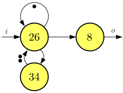
Note, however, that this model is still pessimistic. It has, in contrast to the first model, the correct worst-case throughput, but it predicts a response time for two task executions of 64, while we have seen that it is 60. An exact worst-case model exists in this particular case, shown below, but it need not exist in general. Close approximations can be very large, so they are not commonly applied.

More details about accurate response-time modelling, especially for TDM (Time-Division Multiplex) arbiters, can be found in (Lele, Moreira, and Cuijpers 2012). The key message of this example is that worst-case max-plus-linear models, because of monotonicity, can be used to reason about the performance metrics of a system under worst-case timing assumptions. These metrics then provide bounds on the actual metrics.