June, 2022
A max-plus-linear system may be limited in the number of outputs it can maximally produce per time unit. We call this the of the system. We can study throughput by considering the behavior of a max-plus-linear system for which an unlimited supply of inputs is present at time \(-\infty{}\) and the first event kicks-off at time \(0\). The inputs are then not limiting the progress of the output production and any existing limitations are inherent in the system. Recall Definition 15 that defines the throughput \(\tau{}\) of an event sequence.
The maximal throughput \(\tau{}\) of a max-plus-linear system \(S\) on output \(k\) is equal to \[ \tau{}(S,k) = \tau{}(y_k) \]
where \[ \delta{},\ldots{},\delta{} \mathbin{\stackrel{S}{\longrightarrow}} y_1, \ldots, y_m \]
The throughput \(\tau{}\) of a max-plus-linear system \(S\) is equal to \[ \tau{}(S) = \min_{1\leq{}k\leq{}m} \tau{}(S, k) \]
If the system \(S\) has multiple outputs we consider the maximal throughput of \(S\) to be the lowest throughput among the outputs it produces.
Consider the conveyor belt of Example 7. If we imagine an unlimited supply of boxes waiting to be transported on the belt we can easily compute that the output is equal to \(a(k) = 5+k .\) Thus, the maximal throughput is computed as \[ \tau{} = \lim_{k\rightarrow\infty} \frac{k}{a(k)} = \lim_{k\rightarrow\infty{}} \frac{k}{5+k} = 1 \]
I.e., the maximal throughput of the conveyor belt is equal to 1 box per second.
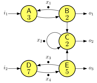
The dataflow graph in Figure 31 has outputs with different throughput. Output \(o_1\) has throughput \(\frac{1}{5}\), as determined by the dependencies between actors A and B. Output \(o_3\) has throughput \(\frac{1}{6}\), determined by the cycle through D and E. finally, output \(o_2\) depends on input from both B and E. The input from E is the slowest and the self-edge cycle on C and the firing duration of 2 of actor C make that C is fast enough to adopt the speed of the actor E. Therefore output \(o_2\) has a throughput of \(\frac{1}{6}\).
The maximal throughput of a system is determined by cyclic dependencies in the system and in terms of the state-space representation, between different elements of the state-vector of the system. Consider the precedence graph in Figure 25. An edge in the graph from node \(x_i\) to node \(x_j\), labelled with \(c\) embodies the constraint that \({\textrm{\bf{}{x}}}(k+1)[j]\geq{}c\otimes{}{\textrm{\bf{}{x}}}(k)[i]\). The edge from \(x_3\) to \(x_2\) implies that \[{\textrm{\bf{}{x}}}(k+1)[2]\geq{}7\otimes{}{\textrm{\bf{}{x}}}(k)[3]\]
The critical cycle shown in red indicates that for all \(k\) \[{\textrm{\bf{}{x}}}(k+1)[1]\geq{}{\textrm{\bf{}{x}}}(k)[2]\] \[{\textrm{\bf{}{x}}}(k+1)[2]\geq{}8\otimes{}{\textrm{\bf{}{x}}}(k)[1]\] and therefore \[{\textrm{\bf{}{x}}}(k+2)[1]\geq{}8\otimes{}{\textrm{\bf{}{x}}}(k)[1]\] and similar for \({\textrm{\bf{}{x}}}[2]\). Therefore, \({\textrm{\bf{}{x}}}(k)[1]\) advances by at least 8 from \(k\) to \(k+2\), so on average at least \(4\) for every increment of \(k\). This limits the throughput to at most \(\frac{1}{4}\), and in general, the throughput for any state element is limited by the critical cycle, the cycle with the maximum cycle mean from which the state element is accessible.
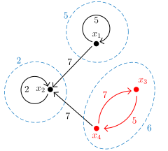
The precedence graph in Figure 32 corresponds to the matrix below, which, in turn, is the state matrix of the dataflow graph of Figure 31. \[ \left[ \begin{array}{cccc} 5 & -\infty{} & -\infty{} & -\infty{} \\ 7 & 2 & -\infty{} & 7 \\ -\infty{} & -\infty{} & -\infty{} & 5 \\ -\infty{} & -\infty{} & 7 & -\infty{} \\ \end{array} \right] \]
The critical cycle is shown in red and has a cycle mean of 6. Clearly, \(x_3\) and \(x_4\) advance at an average rate of 6 time units per iteration. Also \(x_2\) will advance with the same average rate, because there is a path from \(x_3\) (and also from \(x_4\)) to \(x_2\). \(x_1\) on the other hand, does not depend on \(x_3\) or \(x_4\), there is no path from \(x_3\) to \(x_1\). Therefore, \(x_1\) will advance with an average rate of 5 time units per iteration. In general, every element of the state vector will advance, on average, with the rate of the cycle with the largest cycle mean from which it is accessible. In Figure 32, the blue dashed lines show the strongly connected components of the precedence graph. All elements in a strongly connected component must have the same average rate. Every strongly connected component adopts the rate of the slowest strongly connected component from which it is accessible.
The throughput of an output of the system is determined by the slowest state element on which it depends. We can observe from the dataflow graph in Figure 31 that output \(o_1\) depends only on \(x_1\) and therefore has a throughput of \(\frac{1}{5}\). \(o_2\) depends on the tokens, \(\{x_1, x_2, x_3, x_4\}\). \(o_3\) depends on \(\{x_3, x_4\}\). Both outputs therefore adopt the average rate of \(x_3\) and \(x_4\) and have a throughput of \(\frac{1}{6}\).
We can determine the dependencies from the state-space representation. The matrix below is the full state-space matrix of the same system. Recall that the matrix \({\textrm{\bf{}{C}}}\) expresses the direct dependencies between the state vector and the outputs (the first row for \(o_1\), second row for \(o_2\), and third row for \(o_3\)). In general, an output \(y_k\) depends on state-vector element \(x_m\) if there is some state-vector element \(x_l\) such that \({\textrm{\bf{}{C}}}[k,l]\neq{}-\infty{}\) and \(x_l\) is accessible from \(x_m\) in the precedence graph of the state matrix \({\textrm{\bf{}{A}}}\). The afore-mentioned dependencies can now be verified using the state-space model and the precedence graph of Figure 32. \[ \begin{bmatrix}{\textrm{\bf{}{A}}}&{\textrm{\bf{}{B}}}\\{\textrm{\bf{}{C}}}&{\textrm{\bf{}{D}}}\\\end{bmatrix}= \left[ \begin{array}{ccccc|ccc} \!& 5 & -\infty{} & -\infty{} & -\infty{} & 5 & -\infty{} &\! \\ \!& 7 & 2 & -\infty{} & 7 & 7 & -\infty{} &\! \\ \!& -\infty{} & -\infty{} & -\infty{} & 5 & -\infty{} & -\infty{} &\! \\ \!& -\infty{} & -\infty{} & 7 & -\infty{} & -\infty{} & 7 &\! \\ \!& 5 & -\infty{} & -\infty{} & -\infty{} & 5 & -\infty{} &\! \\ \!& 7 & 2 & -\infty{} & 7 & 7 & -\infty{} &\! \\ \!& -\infty{} & -\infty{} & -\infty{} & 5 & -\infty{} & -\infty{} &\! \\ \end{array} \right] \]
Let \(S\) be a max-plus-linear system with state matrix \({\textrm{\bf{}{A}}}\) with largest eigenvalue \(\lambda{}\). If for every element of the state vector there is an output that depends on it, then the maximal throughput of \(S\) is \(\frac{1}{\lambda}\).
If \({\textrm{\bf{}{A}}}\) does not have an eigenvalue, i.e., if its precedence graph has no cycles, then the throughput of \(S\) is not bounded.
Let \(S\) be a max-plus-linear system with state matrix \({\textrm{\bf{}{A}}}\) with largest eigenvalue \(\lambda{}\) and let input sequences \(u_1, \ldots, u_k\) have respective average rates of \(\frac{1}{\mu{}_1}, \ldots, \frac{1}{\mu{}_k}\), then the average rate of the output sequence \(y\) is \(\frac{1}{\lambda{}\oplus{}\mu{}_1\oplus{}\ldots{}\oplus{}\mu{}_k}\).
We have seen that the self-timed execution of a timed dataflow graph can be modelled as a max-plus-linear system using the state-space representation. Therefore, the above results allow us to predict the (maximal) throughput of a dataflow graph under self-timed execution.
Let matrices \({\textrm{\bf{}{A}}}\), \({\textrm{\bf{}{B}}}\), \({\textrm{\bf{}{C}}}\) and \({\textrm{\bf{}{D}}}\) be the state-space representation of a timed dataflow graph \(G\). Let \({\textrm{\bf{}{A}}}\) have largest eigenvalue \(\lambda{}\). Then the maximal throughput of \(G\) is equal to \(\frac{1}{\lambda{}}\). If \(G\) is provided with input event sequences with rates \(\frac{1}{\mu_1}\), , \(\frac{1}{\mu_k}\), then the throughput of the self-timed execution is \(\frac{1}{\lambda{}\oplus{}\mu{}_1\oplus{}\ldots{}\oplus{}\mu{}_k}\).
In Example 20 we have seen that the state matrix of the railroad system is equal to \[ {\textrm{\bf{}{A}}} = \left[ \begin{array}{cccc} -\infty{} & 1 & 3 & -\infty{} \\ 1 & -\infty{} & -\infty{} & -\infty{} \\ 4 & -\infty{} & -\infty{} & 4 \\ 4 & -\infty{} & -\infty{} & 4 \\ \end{array} \right] \]
The following is the corresponding precedence graph assuming the state vector \(\begin{bmatrix}{T_1}~{T_2}~{T_3}~{T_4}\end{bmatrix}^T\).
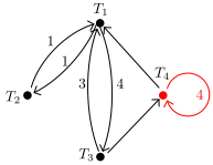
The maximum cycle mean is on the one-step cycle on state variable \(T_4\). All other state variables are accessible from \(T_4\), hence they will also adopt the rate of 4 time units per step. From the state matrices in Example 20 we see that state variables \(T_3\) and \(T_4\) depend on input \(l\), that output \(s\) depends on state variables \(T_2\) and \(T_3\) and that output \(s\) does not directly depend on input \(l\).
Therefore, the throughput of the railroad network is \(\frac{1}{4}\) and the throughput of the output sequence \(s\) will be the minimum of the throughput of the input sequence and the maximum throughput of the railroad network, which is \(\frac{1}{4}\).
In general, the throughput of an output \({\textrm{\bf{}{y}}}[k]\) of a state-space model with given inputs is the minimum of the throughput of the event sequences of the state variables on which it depends and of any inputs, \({\textrm{\bf{}{u}}}[m]\), on which it depends, either directly, according to matrix \({\textrm{\bf{}{D}}}\), or indirectly if any of the state variables on which it depends is accessible from any state variable that depends on \({\textrm{\bf{}{u}}}[m]\).
The output of a max-plus-linear system assumes the throughput of the input provided to the system, or the inherent throughput of the system itself, whichever is the smaller. That immediately tells us that if we make a pipeline of several systems, connecting the output of one system to an input of the next one, that the overall throughput will be the minimum among the throughput values of the individual systems.
Reconsider the wireless channel decoder and its state-space model of Exercise 19. Derive the maximal throughput that the decoder may achieve from its state-space model.
Reconsider the IBC pipeline of Exercise 3. Derive the throughput that this pipeline may achieve from its state-space model.
Reconsider the producer-consumer pipeline of Exercise 7, with explicit input and output.