June, 2022
Equations in max-plus algebra describe relations and systems that are linear. Just like traditional linear systems, it is convenient to use matrix and vector notation to compactly represent sets of equations and transformations involving multiple variables.
A max-plus vector of size \(n\) is a tuple \({\textrm{\bf{}{v}}}\in{}\mathbb{T}^n\) of \(n\) time stamps. It is written as a column of values enclosed by square brackets, e.g., \[\left[\begin{array}{c}{0}\\{-\infty{}}\\\end{array}\right]\in{}\mathbb{T}^2\]
If \({\textrm{\bf{}{v}}}\) and \({\textrm{\bf{}{w}}}\) are two vectors of the same size, we can compute their maximum by applying the additive operator \(\oplus{}\) to corresponding elements, i.e., \(({\textrm{\bf{}{v}}}\oplus{}{\textrm{\bf{}{w}}})[k] = {\textrm{\bf{}{v}}}[k]\oplus{}{\textrm{\bf{}{w}}}[k]\), the result is a vector, \({\textrm{\bf{}{v}}}\oplus{}{\textrm{\bf{}{w}}}\), also of the same size. Recall that, according to the \(\oplus{}\) operator we take the element-wise maximum of the corresponding vector elements.
A vector \({\textrm{\bf{}{v}}}\) can also be delayed by a scalar constant \(c\in\mathbb{T}\). The result is a new vector, \(c\otimes{}{\textrm{\bf{}{v}}}\), which is such that \((c\otimes{}{\textrm{\bf{}{v}}})[k]=c\otimes{}({\textrm{\bf{}{v}}}[k]).\) That means, we get a new vector of the same length where the value \(c\) has been added to each of the elements of the original vector \({\textrm{\bf{}{v}}}\). If one vector is a delayed version of the other, the vectors are called dependent. Otherwise they are independent.
There is a strong analogy between classical linear algebra and max-plus linear algebra. We can also define an inner product between vectors \({\textrm{\bf{}{v}}}\) and \({\textrm{\bf{}{w}}}\) of the same size \(n\). \(({\textrm{\bf{}{v}}}, {\textrm{\bf{}{w}}}) = \bigoplus_{1\leq k\leq n} {\textrm{\bf{}{v}}}[k]\otimes{}{\textrm{\bf{}{w}}}[k]\). It is easy to see that \(({\textrm{\bf{}{v}}}, {\textrm{\bf{}{w}}})=({\textrm{\bf{}{w}}}, {\textrm{\bf{}{v}}})\). It is often written as \({\textrm{\bf{}{v}}}^T {\textrm{\bf{}{w}}}\) because of the similarity with matrix multiplication.
The maximum and delay on max-plus vectors \({\textrm{\bf{}{v}}}\) and \({\textrm{\bf{}{w}}}\) are defined as follows: \[({\textrm{\bf{}{v}}}\oplus{}{\textrm{\bf{}{w}}})[k] = {\textrm{\bf{}{v}}}[k]\oplus{}{\textrm{\bf{}{w}}}[k]\] \[(c\otimes{}{\textrm{\bf{}{v}}})[k]=c\otimes{}({\textrm{\bf{}{v}}}[k])\]
Vectors \({\textrm{\bf{}{v}}}\) and \({\textrm{\bf{}{w}}}\) are called dependent if there exists \(c\in{}\mathbb{T}\) such that \(c\otimes{}{\textrm{\bf{}{v}}} = {\textrm{\bf{}{w}}}\) or \({\textrm{\bf{}{v}}} = c\otimes{}{\textrm{\bf{}{w}}}\).
The inner product \(({\textrm{\bf{}{v}}}, {\textrm{\bf{}{w}}})\) between vectors \({\textrm{\bf{}{v}}}\) and \({\textrm{\bf{}{w}}}\) is \[({\textrm{\bf{}{v}}}, {\textrm{\bf{}{w}}}) = \bigoplus_{1\leq k\leq n} {\textrm{\bf{}{v}}}[k]\otimes{}{\textrm{\bf{}{w}}}[k] .\]
A max-plus matrix of size \(n\) by \(m\) is a table \({\textrm{\bf{}{A}}}\in{}\mathbb{T}^{n\times{}m}\) of \(n\) rows and \(m\) columns containing time stamps. It is written as a table of values enclosed by square brackets, e.g., \[\begin{bmatrix}{0} & {-\infty{}}\\{-\infty{}} & {0}\\\end{bmatrix}\in{}\mathbb{T}^{2\times{}2}\]
A max-plus matrix \({\textrm{\bf{}{A}}}\in{}\mathbb{T}^{m\times{}n}\) can be multiplied with a vector \({\textrm{\bf{}{v}}}\in{}\mathbb{T}^{n}\). The result is a vector \({\textrm{\bf{}{w}}}\in{}\mathbb{T}^{m}\) such that \[ {\textrm{\bf{}{w}}}[k] = \bigoplus_{1\leq{}i\leq{}n} {\textrm{\bf{}{A}}}[k,i]\otimes{}{\textrm{\bf{}{v}}}[i] \]
It is written as \({\textrm{\bf{}{w}}}={\textrm{\bf{}{A}}}{\textrm{\bf{}{v}}}\).
A max-plus matrix \({\textrm{\bf{}{A}}}\in{}\mathbb{T}^{m\times{}n}\) can be multiplied with a matrix \({\textrm{\bf{}{B}}}\in{}\mathbb{T}^{n\times{}k}\). The result is a matrix \({\textrm{\bf{}{C}}}\in{}\mathbb{T}^{m\times{}k}\) such that \[ {\textrm{\bf{}{C}}}[i,j] = \bigoplus_{1\leq{}l\leq{}n} {\textrm{\bf{}{A}}}[i,l]\otimes{}{\textrm{\bf{}{B}}}[l,j] \]
It is written as \({\textrm{\bf{}{C}}}={\textrm{\bf{}{A}}}{\textrm{\bf{}{B}}}\).
A vector norm that is convenient in max-plus linear algebra is the max norm, a measure that assigns to a vector the maximum of the elements in the vector.
The (max) norm of a max-plus vector \({\textrm{\bf{}{v}}}\) of size \(n\) is \[ \left|{{\textrm{\bf{}{v}}}}\right| = \bigoplus_{1\leq k \leq n} {\textrm{\bf{}{v}}}[k] \]
A vector \({\textrm{\bf{}{v}}}\) is called normal if \(\left|{{\textrm{\bf{}{v}}}}\right|=0\).
If \({\textrm{\bf{}{v}}}\) is a max-plus vector with a norm \(\left|{{\textrm{\bf{}{v}}}}\right| \neq -\infty{}\), then the normalized vector of \({\textrm{\bf{}{v}}}\) is the vector \((-\left|{{\textrm{\bf{}{v}}}}\right|)\otimes{}{\textrm{\bf{}{v}}}\). The norm of a normalized vector is \(0\), i.e., it is normal.
Note that a vector \({\textrm{\bf{}{v}}}\) with norm \(-\infty{}\) cannot be normalized, as there exists no constant \(c\in{}\mathbb{T}\) such that \(|c\otimes{}{\textrm{\bf{}{v}}}| = 0\). A normalized vector has no positive entries. All of its entries are \(0\), negative numbers, or \(-\infty{}\).
Matrix-vector and matrix-matrix multiplication in max-plus algebra are linear. For all \(c,d\in{}\mathbb{T}\), vectors \({\textrm{\bf{}{x}}}, {\textrm{\bf{}{y}}}\) and matrices \({\textrm{\bf{}{A}}}, {\textrm{\bf{}{B}}}, {\textrm{\bf{}{C}}}\), the following equations hold (provided the matrices and vectors are of appropriate sizes for the operations performed) \[ \begin{aligned} {\textrm{\bf{}{A}}}(c\otimes{}{\textrm{\bf{}{x}}}\oplus{}d\otimes{}{\textrm{\bf{}{y}}}) &= c\otimes{}({\textrm{\bf{}{A}}}{\textrm{\bf{}{x}}})\oplus{}d\otimes{}({\textrm{\bf{}{A}}}{\textrm{\bf{}{y}}})\\ {\textrm{\bf{}{A}}}(c\otimes{}{\textrm{\bf{}{B}}}\oplus{}d\otimes{}{\textrm{\bf{}{C}}}) &= c\otimes{}({\textrm{\bf{}{A}}}{\textrm{\bf{}{B}}})\oplus{}d\otimes{}({\textrm{\bf{}{A}}}{\textrm{\bf{}{C}}})\\ \end{aligned} \]
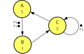
Dataflow graphs are max-plus-linear systems and their behavior can be expressed in max-plus algebra. In particular, the time stamps of events, such as input arrivals, token productions, actor firings and output productions can be related to each other with equations in max-plus algebra. Such sets of equations are conveniently captured using matrices and vectors. We illustrate this with the following example.
Consider the dataflow graph in Figure 20. It has three initial tokens. We assume the tokens have time stamps indicating their first availability times. These time stamps are indicated in Figure 20 as \(x_1\), \(x_2\) and \(x_3\). The tokens time stamped \(x_1\) and \(x_2\) are on the same channel, such that the token with time stamp \(x_1\) is the first to be consumed by actor \(B\). We know that after one firing of each of the actors the configuration of tokens on the channels will return to the same state, but with new time stamps. We can derive equations for those new time stamps under self-timed execution as follows. Actor \(B\) will fire at time \(x_1\). This firing completes at time \(x_1+1=1\otimes{}x_1\). The firing of actor \(C\) needs the token produced by \(B\) as well as the token on its self-edge with time stamp \(x_3\). Therefore, \(C\) starts its firing at \(\max(1\otimes{}x_1, x_3)=1\otimes{}x_1\oplus{}x_3\) and completes the firing 2 time units later, at \(3\otimes{}x_1\oplus{}2\otimes{}x_3\). At this time, the new token on the self-edge of \(C\) is produced, so it gets the time stamp \(x_3'= 3\otimes{}x_1\oplus{}2\otimes{}x_3\). Finally, actor \(A\) starts its firing at the same time that \(C\) finishes and \(A\) itself finishes 5 time units later at \(8\otimes{}x_1\oplus{}7\otimes{}x_3\). Therefore, we have \(x_2'= 8\otimes{}x_1\oplus{}7\otimes{}x_3\). The token with time stamp \(x_2\) was not consumed in the process, but it has moved up to the position of the first token to be consumed next by \(B\); therefore, we have \(x_1'= x_2 = 0\otimes{}x_2\). Summarizing, we have the following equations. \[ \begin{aligned} x_1'&= \phantom{8\otimes{}x_1\oplus{}}0\otimes{}x_2\\ x_2'&= 8\otimes{}x_1\phantom{\oplus{}0\otimes{~}x_2\oplus{}}7\otimes{}x_3\\ x_3'&= 3\otimes{}x_1\phantom{\oplus{}0\otimes{~}x_2\oplus{}}2\otimes{}x_3\\ \end{aligned} \]
We have formatted the equations above in such a way that it is easy to see that we can collect these equations in the form of a matrix-vector equation: \[ \begin{bmatrix}{x_1'}\\{x_2'}\\{x_3'}\end{bmatrix} = \begin{bmatrix}{-\infty{}}&{0}&{-\infty{}}\\{8}&{-\infty{}}&{7}\\{3}&{-\infty{}}&{2}\\\end{bmatrix} \begin{bmatrix}{x_1}\\{x_2}\\{x_3}\end{bmatrix} \]
Note how in case there is no dependency from an old time stamp to a new time stamp, we fill the matrix with \(-\infty{}\) at the corresponding location. Considering the fact that the dataflow graph actors keep firing over and over again, we can associate with the sequences of time stamps they produce the event sequences \(x_1(k)\), \(x_2(k)\) and \(x_3(k)\). The equation can then recursively be used to compute the sequence of all tokens as follows. \[ \begin{bmatrix}{x_1(k+1)}\\{x_2(k+1)}\\{x_3(k+1)}\end{bmatrix} = \begin{bmatrix}{-\infty{}}&{0}&{-\infty{}}\\{8}&{-\infty{}}&{7}\\{3}&{-\infty{}}&{2}\\\end{bmatrix} \begin{bmatrix}{x_1(k)}\\{x_2(k)}\\{x_3(k)}\end{bmatrix} \]
In short, with \({\textrm{\bf{}{x}}}(k)=\begin{bmatrix}{x_1(k)}\\{x_2(k)}\\{x_3(k)}\end{bmatrix}\) and \({\textrm{\bf{}{G}}}=\begin{bmatrix}{-\infty{}}&{0}&{-\infty{}}\\{8}&{-\infty{}}&{7}\\{3}&{-\infty{}}&{2}\\\end{bmatrix}\), we have \[ {\textrm{\bf{}{x}}}(k+1)={\textrm{\bf{}{G}}}{\textrm{\bf{}{x}}}(k) \]
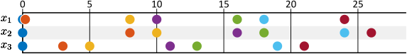
The resulting sequences of time stamps are shown in Figure 21.
We can use the result, for example, to answer questions about makespan, such as what is the makespan of the self-timed execution of 6 iterations of the dataflow graph? In this example, we know that the last firing completes with the production of a token, so we can express the makespan as \[ M = \left|{{\textrm{\bf{}{G}}}^{6}{\bf{0}}}\right|=26 \]
The result can be verified on Figure 21 as the norm of the last (red) vector.
Reconsider the producer-consumer pipeline of Exercise 2 with function \(f_2\) for the filter actor \(F\).