June, 2022
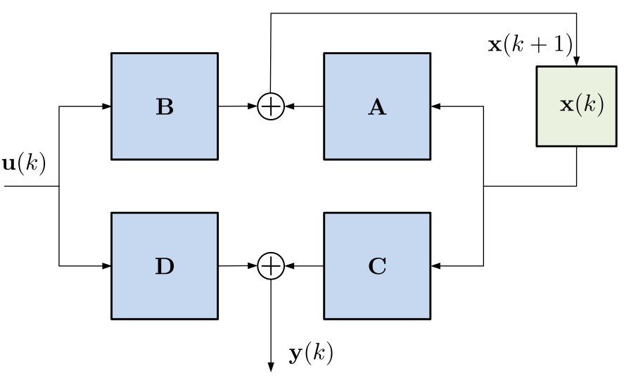
Max-plus-linear event systems are often described with linear-algebra equations. The system is assumed to have an internal state that can be captured as a vector \({\textrm{\bf{}{x}}}\in\mathbb{T}^{n}\) of \(n\) time stamps, for some \(n\in\mathbb{N}\). The inputs to the event system are collected as a sequence of vectors \({\textrm{\bf{}{u}}}(k)\), where vector \({\textrm{\bf{}{u}}}(k)\) contains the \(k\)-th sample from each of the input event sequences. In a similar way, the outputs of the system are collected in a sequence \({\textrm{\bf{}{y}}}(k)\) of vectors. As the system operates, the next state, \({\textrm{\bf{}{x}}}(k+1)\) may depend on the current inputs \({\textrm{\bf{}{u}}}(k)\) and the current state, \({\textrm{\bf{}{x}}}(k)\). The outputs \({\textrm{\bf{}{y}}}(k)\) may also depend on the current state and the current inputs. Note that the current state and current input refers to the event index, not to the point in time. The various dependencies, being linear, can be characterized by matrices. Such a description of a max-plus-linear system is called a state-space representation.
A single-rate max-plus linear and index-invariant system with finite-dimensional state can be characterized using the following set of max-plus-linear matrix-vector equations. \[ \left\lbrace \begin{aligned} {\textrm{\bf{}{x}}}(k+1) &= {\textrm{\bf{}{A}}} {\textrm{\bf{}{x}}}(k) \oplus{} {\textrm{\bf{}{B}}} {\textrm{\bf{}{u}}}(k) \\ {\textrm{\bf{}{y}}}(k) &= {\textrm{\bf{}{C}}} {\textrm{\bf{}{x}}}(k) \oplus{} {\textrm{\bf{}{D}}} {\textrm{\bf{}{u}}}(k) \\ \end{aligned} \right. \]
The state-space representation is graphically represented in Figure 28. Matrix \({\textrm{\bf{}{A}}}\) is called the state matrix (also called system matrix). \({\textrm{\bf{}{B}}}\) is the input matrix. \({\textrm{\bf{}{C}}}\) is the output matrix and \({\textrm{\bf{}{D}}}\) is the feed-forward matrix.
The conveyor belt of Example 9 can be captured using the state-space representation. It requires only a single state variable, \(x\), so its state vector has length \(n=1\). The state of the system represents all information from the past that is needed to describe its impact on the future. Let \(x(k)\) be the time stamp at which the previous object has passed the entrance of the belt, i.e., the earliest time that the next object can be placed on the belt. With this definition we need to describe the four dependencies.
The state-space equations for the conveyor belt are therefore as follows. \[ \left\lbrace \begin{aligned} x(k+1) &= \frac{d}{v} \otimes{}x(k) \oplus{} \frac{d}{v} \otimes{}i(k) \\ o(k) &= \frac{l}{v}\otimes{} x(k) \oplus{} \frac{l}{v}\otimes{}i(k) \\ \end{aligned} \right. \]
The state-space equations are often collected into a single matrix-vector equation by collecting the produced vectors \({\textrm{\bf{}{x}}}(k+1)\) and \({\textrm{\bf{}{y}}}(k)\) into a single vector and similarly the input vectors \({\textrm{\bf{}{x}}}(k)\) and \({\textrm{\bf{}{u}}}(k)\) into a single vector. We obtain the equation below. \[ \left[\begin{array}{c}{{\textrm{\bf{}{x}}}(k+1)}\\{{\textrm{\bf{}{y}}}(k)}\\\end{array}\right] = \begin{bmatrix}{\textrm{\bf{}{A}}}&{\textrm{\bf{}{B}}}\\{\textrm{\bf{}{C}}}&{\textrm{\bf{}{D}}}\\\end{bmatrix} \left[\begin{array}{c}{{\textrm{\bf{}{x}}}(k)}\\{{\textrm{\bf{}{u}}}(k)}\\\end{array}\right] \]
Verify that the result is indeed the same.
The state-space matrices define the dependencies of the next-state variables and the outputs on the current state variables and the inputs.
The state-space representation can also be used to describe any timed dataflow graph. Dataflow graphs have a natural definition of their internal state, namely the collection of the time stamps of all the tokens in the graph between iterations of the graph. Note that we have in fact already used such vectors in Section 6.2.
The state-space matrices for a deadlock-free single-rate dataflow graph can be computed with a symbolic simulation method, very similar to Algorithm 1. The method is presented in Algorithm 2 below. The changes compared to Algorithm 1 are indicated in red.
Perform the following steps.
The state vector consists of the time stamps of the tokens, \({\textrm{\bf{}{x}}}=[T_1, T_2, T_3, T_4]^T\).
We perform a symbolic simulation as in Example 14, but with the generalizations of Algorithm 2 to obtain the state-space equations.
For the symbolic time stamps, we include the input variable \(l\) representing the arrival \(l(k)\) of a train on the input. We also assign the input a symbolic time stamp vector, which becomes \({{\textrm{\bf{}{i}}}_{5}}\). (Recall that \({{\textrm{\bf{}{i}}}_{1}}\), , \({{\textrm{\bf{}{i}}}_{4}}\) represent the four initial tokens.)
During the symbolic simulation we follow the same sequence of actor firings as in Example 14. The symbolic time-stamp vectors for the actor firing starts and completions are now of length 5, including the input.
| actor | symbolic start | symbolic completion |
|---|---|---|
| TEM | \([ ~ {-\infty{}} ~{-\infty{}} ~{-\infty{}} ~0 ~{-\infty{}}]^{T}\) | \([ ~ {-\infty{}} ~{-\infty{}} ~{-\infty{}} ~2 ~{-\infty{}}]^{T}\) |
| MST | \([ ~ {-\infty{}} ~{-\infty{}} ~{-\infty{}} ~2 ~0]^{T}\) | \([ ~ {-\infty{}} ~{-\infty{}} ~{-\infty{}} ~2 ~0]^{T}\) |
| TME | \([ ~ {-\infty{}} ~{-\infty{}} ~{-\infty{}} ~2 ~0]^{T}\) | \([ ~ {-\infty{}} ~{-\infty{}} ~{-\infty{}} ~4 ~2]^{T}\) |
| THA | \([ ~ {-\infty{}} ~0 ~{-\infty{}} ~{-\infty{}} ~{-\infty{}}]^{T}\) | \([ ~ {-\infty{}} ~1 ~{-\infty{}} ~{-\infty{}} ~{-\infty{}}]^{T}\) |
| TAH | \([ ~ 0 ~{-\infty{}} ~{-\infty{}} ~{-\infty{}}~{-\infty{}} ]^{T}\) | \([ ~ 1 ~{-\infty{}} ~{-\infty{}} ~{-\infty{}} ~{-\infty{}}]^{T}\) |
| THG | \([ ~ 1 ~{-\infty{}} ~{-\infty{}} ~{-\infty{}} ~{-\infty{}}]^{T}\) | \([ ~ 1 ~{-\infty{}} ~{-\infty{}} ~{-\infty{}} ~{-\infty{}}]^{T}\) |
| THE | \([ ~ 1 ~{-\infty{}} ~{-\infty{}} ~{-\infty{}} ~{-\infty{}}]^{T}\) | \([ ~ 4 ~{-\infty{}} ~{-\infty{}} ~{-\infty{}}~{-\infty{}} ]^{T}\) |
| EHV | \([ ~ 4 ~{-\infty{}} ~{-\infty{}} ~4 ~2]^{T}\) | \([ ~ 4 ~{-\infty{}} ~{-\infty{}} ~4 ~2]^{T}\) |
| TEA | \([ ~ {-\infty{}} ~{-\infty{}} ~0 ~{-\infty{}} ~{-\infty{}}]^{T}\) | \([ ~ {-\infty{}} ~{-\infty{}} ~3 ~{-\infty{}} ~{-\infty{}}]^{T}\) |
| AMS | \([ ~ {-\infty{}} ~1 ~3 ~{-\infty{}} ~{-\infty{}}]^{T}\) | \([ ~ {-\infty{}} ~1 ~3 ~{-\infty{}} ~{-\infty{}}]^{T}\) |
| TAS | \([ ~ {-\infty{}} ~1 ~3 ~{-\infty{}}~{-\infty{}} ]^{T}\) | \([ ~ {-\infty{}} ~2 ~4 ~{-\infty{}} ~{-\infty{}}]^{T}\) |
Token \(T_1\) is produced by actor AMS, \(T_2\) by THG, \(T_3\) and \(T_4\) by EHV. Collecting the symbolic time-stamp vectors for the new tokens as the rows of the matrix gives the following result. \[ \begin{bmatrix}{{\textrm{\bf{}{A}}}}~{{\textrm{\bf{}{B}}}}\end{bmatrix}= \left[ \begin{array}{cccc|c} -\infty{} & 1 & 3 & -\infty{} & -\infty{} \\ 1 & -\infty{} & -\infty{} & -\infty{} & -\infty{} \\ 4 & -\infty{} & -\infty{} & 4 & 2 \\ 4 & -\infty{} & -\infty{} & 4 & 2 \\ \end{array} \right] \]
During the symbolic simulation we have also recorded the production of the output \(s\), which coincides with the completion of the firing of actor TAS. This gives us the matrices \({\textrm{\bf{}{C}}}\) and \({\textrm{\bf{}{D}}}\). \[ \begin{bmatrix}{{\textrm{\bf{}{C}}}}~{{\textrm{\bf{}{D}}}}\end{bmatrix}= \left[ \begin{array}{cccc|c} -\infty{} & 2 & 4 & -\infty{} & -\infty{} \\ \end{array} \right] \]
Note that because there is only one input, \({\textrm{\bf{}{B}}}\) and \({\textrm{\bf{}{D}}}\) have only one column, and because there is only one output, \({\textrm{\bf{}{C}}}\) and \({\textrm{\bf{}{D}}}\) have only one row. Thus the feed-forward matrix \({\textrm{\bf{}{D}}}\) contains only one element, \(-\infty{}\), which indicates that there is no dependency of \(s(k)\) on \(l(k)\).
In the context of the state-space representation of a max-plus-linear system, we can determine the impulse response of a selected input \(k\) as follows. We create a sequence \({\textrm{\bf{}{u}}}(k)\) of input vectors such that the sequence \({\textrm{\bf{}{u}}}(m)[k]\) is the impulse sequence \(\delta{}\) and \({\textrm{\bf{}{u}}}(m)[n] = \epsilon{}\) for all \(n\neq{}k\). In terms of the sequence of input vectors, we have \({\textrm{\bf{}{u}}}(0) = {{\textrm{\bf{}{i}}}_{k}}\) and \({\textrm{\bf{}{u}}}(k)=\bf{\epsilon}\) for all \(k>0\). (Recall that \(\bf{\epsilon}\) is the vector containing only \(-\infty{}\) as its elements.) We then consider the corresponding sequence \({\textrm{\bf{}{y}}}(k)\) of output vectors, starting from the initial state \({\textrm{\bf{}{x}}}(0)=\bf{\epsilon}\), as the impulse response. Very often we also want to observe the response of the impulse input on the sequence \({\textrm{\bf{}{x}}}(k)\) of state vectors. In that sense, the sequence \({\textrm{\bf{}{x}}}(k)\) is included when we talk about the impulse response of a certain input.
Just like dataflow graphs can be subject to self-timed scheduling, or can be executed according to a prescribed schedule (Definition 2), we can also define a schedule for max-plus-linear systems in state-space representation. In this case, we prescribe the sequence of state vectors that are used for every iteration of the system. Such schedules can only be followed if they are valid, i.e., if all constraints, input constraints and internal constraints, are met.
A schedule \({\bf{\sigma{}}}\) of a max-plus-linear system in state-space representation with state matrix \({\textrm{\bf{}{A}}} \in \mathbb{T}^{n\times{}n}\) is a sequence of vectors from \(\mathbb{T}^{n}\). The schedule is valid for a given input sequence \({\textrm{\bf{}{u}}}(k)\) if for all \(k\in\mathbb{N}\), \[ {\textrm{\bf{}{A}}}{\bf{\sigma{}}}(k) \oplus{} {\textrm{\bf{}{B}}}{\textrm{\bf{}{u}}}(k) \leq{}{\bf{\sigma{}}}(k+1) \]
In general, we describe the execution that follows from a given schedule (valid or not valid) as follows.
The sequence of system states and outputs of the execution of a max-plus-linear system with state-space matrices \({\textrm{\bf{}{A}}}\), \({\textrm{\bf{}{B}}}\), \({\textrm{\bf{}{C}}}\) and \({\textrm{\bf{}{D}}}\) with inputs \({\textrm{\bf{}{u}}}(k)\) and schedule \({\bf{\sigma{}}}(k)\) is defined by the following equations. \[ {\textrm{\bf{}{x}}}(0) = {\bf{\sigma{}}}(0) \] \[ {\textrm{\bf{}{x}}}(k+1) = {\textrm{\bf{}{A}}}{\textrm{\bf{}{x}}}(k) \oplus{} {\textrm{\bf{}{B}}}{\textrm{\bf{}{u}}}(k)\oplus{} {\bf{\sigma{}}}(k+1) \] \[ {\textrm{\bf{}{y}}}(k)={\textrm{\bf{}{C}}}{\textrm{\bf{}{x}}}(k)\oplus{} {\textrm{\bf{}{D}}}{\textrm{\bf{}{u}}}(k) \]
For all \(k\in\mathbb{N}\), \({\bf{\sigma{}}}(k)\leq{}{\textrm{\bf{}{x}}}(k)\), and if the schedule is valid \({\textrm{\bf{}{x}}}(k)={\bf{\sigma{}}}(k)\)
The impulse-response analysis discussed in Example 12 can also be applied to investigate how disturbances in the operation impact the schedule or execution. For example, to study the impact of a late arriving input, or an extended duration of an operation.
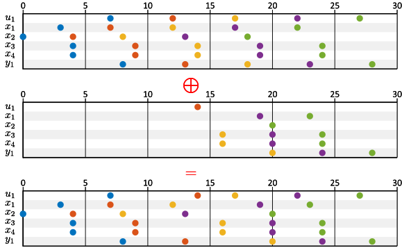
Consider the periodic train schedule shown in the top trace in Figure 30 in the form of a sequence of state vectors. Recall that from those state vectors and from the input sequence, all details of the trains operating in a self-timed fashion, can be reconstructed.
This particular periodic train schedule operates at a period of five hours, although a periodic schedule with a period of four hours also exists (see Figure 27), i.e., it has a bit of slack. Let \(\overline{{\textrm{\bf{}{p}}}}\) be the sequence of state vectors in the periodic schedule of Figure 30. Note that the state vectors are a valid schedule (see Definition 35) if we assume that all inputs arrive early enough, i.e., for all \(k\in\mathbb{N}\), \[ {\textrm{\bf{}{A}}} \overline{{\textrm{\bf{}{p}}}}(k) \leq{} \overline{{\textrm{\bf{}{p}}}}(k+1) \]
In words, this means that all trains return, at the end of an iteration, in time to depart according to the next scheduled departure times. We assume that within an iteration of the schedule all trains depart as soon as possible.
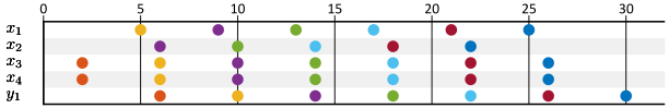
Assume now that we want to study the impact on the schedule from a delay of two hours of the second train from Liège. I.e., it arrives at \(14.00\) hours instead of at \(12.00\) hours. We can use the impulse response on the state vectors, which is shown in Figure 29. Let \(\overline{{\textrm{\bf{}{h}}}}\) be the impulse-response vector sequence of Figure 29. (Note that Figure 29 additionally shows the impulse response on the output.) \[ \overline{{\textrm{\bf{}{h}}}} = \begin{bmatrix}{-\infty{}}\\{-\infty{}}\\{-\infty{}}\\{-\infty{}}\end{bmatrix}, \begin{bmatrix}{-\infty{}}\\{-\infty{}}\\{2}\\{2}\end{bmatrix}, \begin{bmatrix}{5}\\{-\infty{}}\\{6}\\{6}\end{bmatrix}, \begin{bmatrix}{9}\\{6}\\{10}\\{10}\end{bmatrix}, \begin{bmatrix}{13}\\{10}\\{14}\\{14}\end{bmatrix}, \ldots \]
The impulse response, by definition, represents the impact of the first train arriving at time 0. It is easily adapted to the impact of the second train arriving at time \(14\) by an index delay of one sample and a time delay of \(14\), i.e., \(14\otimes{}{{\overline{{\textrm{\bf{}{h}}}}}^{1}}\), which is: \[ 14\otimes{}{{\overline{{\textrm{\bf{}{h}}}}}^{1}} = \begin{bmatrix}{-\infty{}}\\{-\infty{}}\\{-\infty{}}\\{-\infty{}}\end{bmatrix}, \begin{bmatrix}{-\infty{}}\\{-\infty{}}\\{-\infty{}}\\{-\infty{}}\end{bmatrix}, \begin{bmatrix}{-\infty{}}\\{-\infty{}}\\{16}\\{16}\end{bmatrix}, \begin{bmatrix}{19}\\{-\infty{}}\\{20}\\{20}\end{bmatrix}, \begin{bmatrix}{23}\\{20}\\{24}\\{24}\end{bmatrix}, \begin{bmatrix}{27}\\{24}\\{28}\\{28}\end{bmatrix}, \ldots \]
This sequence is shown in the second trace in Figure 30.
The new train schedule can then be computed as the superposition (i.e., the maximum, \(\oplus{}\)) of the original schedule and the response to the delayed train: \[ \overline{{\textrm{\bf{}{p}}}}\oplus{} 14\otimes{}{{\overline{{\textrm{\bf{}{h}}}}}^{1}} \]
The result is shown in the bottom trace in Figure 30. We see that the third state vector is impacted by the delay, elements of the state are delayed by two time units. The fourth state vector is also impacted, but by one time unit only, and after that the schedule returns to the planned schedule \(\overline{{\textrm{\bf{}{p}}}}\). In terms of the outputs, the trains arriving at Schiphol, we see that the third train is delayed by two hours, the fourth train by one hour and subsequent trains are again on time.
Consider the following variant of the wireless channel decoder.
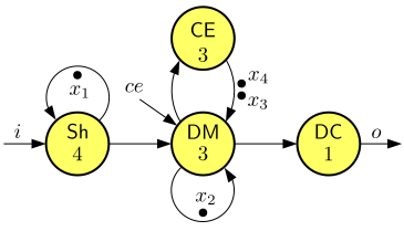
The model is a variant of the model of Exercise 1, where, for simplicity, we omitted two self-edges. (You may check that the omitted self-edges did not impact the timing of the actor firings.) Because we want to investigate the effect of the availability of channel-estimation information on the timing of decoding output, we added a \(ce\) input to actor DM, in line with the construction explained after Theorem 3.