
June, 2022
In Example 13 and Exercise 13, we have derived a matrix equation that captures the relation between subsequent vectors of time stamps of the initial tokens of the graph in subsequent iterations of the dataflow graph. In both cases, all the relevant events have time stamps that can be expressed as max-plus-linear combinations of the time stamps of the initial tokens in the dataflow graph. This is in fact true in general and we exploit this property to develop a general method to compute the max-plus matrix for a deadlock-free single-rate or consistent multi-rate dataflow graph.
Let \(x_1, x_2, \ldots, x_n\) be a finite set of variables that represent time stamps. An expression of the form \[ a_1\otimes{}x_1\oplus{}a_2\otimes{}x_2\oplus{}\ldots \oplus{}a_n\otimes{}x_n \]
that represents a max-plus-linear combination of the given variables for constants \(a_1, a_2, \ldots, a_n\in{}\mathbb{T}\) is called a symbolic time stamp.
A symbolic time stamp is referred to as symbolic, because it represents a time stamp, but not as a value, but as an expression in terms of variables. Note that any symbolic time stamp that depends on only a strict subset of the variables can still be expressed as a symbolic time stamp on the full set of variables using \(-\infty{}\) as the corresponding coefficient for any of the unused variables. For example, \(2\otimes{}x_2 = -\infty{}\otimes{}x_1\oplus{}2\otimes{}x_2\).
We are often working with a number of symbolic time stamps referring to the same, fixed, set of variables, in which case only the coefficients vary. The coefficients can be conveniently collected in a vector.
A symbolic time-stamp vector for a set \(x_1, x_2, \ldots, x_n\) of variables is a vector \({\textrm{\bf{}{t}}}\in{}\mathbb{T}^n\). It represents the symbolic time stamp \[ {\textrm{\bf{}{t}}}[1]\otimes{}x_1\oplus{}\ldots{}\oplus{}{\textrm{\bf{}{t}}}[n]\otimes{}x_n \]
Note that the symbolic time stamp represented by the symbolic time-stamp vector \({\textrm{\bf{}{t}}}\) can be expressed using the vector inner product as \(({\textrm{\bf{}{t}}}, [x_1~ \ldots{}~x_n]^T).\)
Various operations on symbolic time stamps can be performed directly on the symbolic time-stamp vectors that represent them. The results we need are presented below.
Let \({\textrm{\bf{}{t}}}_1\) be a symbolic time-stamp vector for the symbolic time stamp \(e_1\) on the time stamp variables \(x_1, \ldots, x_n\), \({\textrm{\bf{}{t}}}_2\) be a symbolic time-stamp vector for the symbolic time stamp \(e_2\) and \(c\in{}\mathbb{T}\). Then the following results hold.
We can now define a general method to compute for a single-rate dataflow graph a max-plus matrix that expresses the relation between the time stamps of the tokens in the graph before and after the execution of an iteration of the graph (one firing of each of the actors). It is a generalization of the method we used in Example 13 and Exercise 13.
The max-plus matrix for a single-rate dataflow graph without inputs can be constructed with the following procedure. Note that outputs do not influence the behavior of the graph and do not need to be considered. We will see in Section 10.2 how inputs and outputs can be included.
Perform the following steps.
Note that during the procedure, it is always possible to find an actor that is enabled and has not fired until all actors have fired if and only if the graph is deadlock free.
It may happen that some initial tokens in the graph have not been produced or consumed during the symbolic simulation. In particular, this happens precisely on the channels with two or more initial tokens from which one will be consumed and onto which one new token will be produced, like on the example channel below (and in Example 13). In this case, \(x_1\) is consumed during the simulation, but \(x_2\) is not. A new token is also produced onto the channel during the simulation. The token \(x_2\) from the initial state has now become \(x_1\). The newly produced token becomes the new \(x_2\). Therefore, the symbolic time stamp \({\textrm{\bf{}{t}}}_1\) for \(x_1\) at the end of the simulation is equal to the initial symbolic time stamp \({\textrm{\bf{}{t}}}_2\) of \(x_2\) at the start of the simulation, i.e., \({{\textrm{\bf{}{i}}}_{2}}\).
During symbolic simulation, we can record the symbolic time stamps and symbolic time-stamp vectors for any of the events that occur during the self-timed execution of the dataflow graph, not only for the produced tokens. In particular, we can record the start times and completion times of actor firings. The actor firing that consumes the tokens with symbolic time-stamp vectors \({\textrm{\bf{}{t}}}_1, \ldots, {\textrm{\bf{}{t}}}_m\) starts its firing at the time represented by: \[ {\textrm{\bf{}{t}}}_a^{\mathit{start}} = \bigoplus_{1\leq i\leq m} {\textrm{\bf{}{t}}}_i \]
The symbolic time-stamp vector of the completion of an actor firing is: \[ {\textrm{\bf{}{t}}}_a^{\mathit{completion}} = e(a)\otimes{} {\textrm{\bf{}{t}}}_a^{\mathit{start}} \]
During the symbolic-simulation procedure we can therefore also produce the matrices \({\textrm{\bf{}{H}}}^s\) and \({\textrm{\bf{}{H}}}^c\), where the rows of \({\textrm{\bf{}{H}}}^s\) are the symbolic time-stamp vectors of all actor-firing start times and similarly the rows of \({\textrm{\bf{}{H}}}^c\) are the symbolic time-stamp vectors of all actor-firing completion times.
If we know the concrete time stamps of the tokens in the graph in the form of the vector \({\textrm{\bf{}{x}}}\), we can directly compute a vector \({\textrm{\bf{}{s}}}\) with all the concrete actor-firing start times and a vector \({\textrm{\bf{}{c}}}\) with all the concrete actor-firing completion times in an iteration as: \[ {\textrm{\bf{}{s}}} = {\textrm{\bf{}{H}}}^s{\textrm{\bf{}{x}}},~~ {\textrm{\bf{}{c}}} = {\textrm{\bf{}{H}}}^c{\textrm{\bf{}{x}}} \]
And as we use the max-plus matrix \({\textrm{\bf{}{G}}}\) to compute the sequence \({\textrm{\bf{}{x}}}(k)\) of time stamp-vectors using the equation \({\textrm{\bf{}{x}}}(k+1)={\textrm{\bf{}{G}}}{\textrm{\bf{}{x}}}(k)\), we can compute all actor-firing start and completion times as: \[ {\textrm{\bf{}{s}}}(k) = {\textrm{\bf{}{H}}}^s{\textrm{\bf{}{x}}}(k),~~ {\textrm{\bf{}{c}}}(k) = {\textrm{\bf{}{H}}}^c{\textrm{\bf{}{x}}}(k) \]
We can use this, for example, to generate a Gantt-chart visualization (Alizadeh Ara et al. 2017), as it is done in the CMWB.
In the railroad-network dataflow graph of Figure 7, we have four initial tokens \(T_1\), , \(T_4\). We label these with the symbolic time-stamp vectors \({{\textrm{\bf{}{i}}}_{1}}\), \(\ldots\), \({{\textrm{\bf{}{i}}}_{4}}\).
For this example, we ignore the input and output of the network. During the symbolic simulation, we can execute the actors in the order given in the table below. We find the corresponding symbolic time-stamp vectors for the actor firing starts and completions.
| actor | symbolic start | symbolic completion |
|---|---|---|
| TEM | \([ ~{-\infty{}} ~{-\infty{}} ~{-\infty{}} ~0 ]^{T}\) | \([ ~{-\infty{}} ~{-\infty{}} ~{-\infty{}} ~2 ]^{T}\) |
| MST | \([ ~ {-\infty{}} ~{-\infty{}} ~{-\infty{}} ~2 ]^{T}\) | \([ ~ {-\infty{}} ~{-\infty{}} ~{-\infty{}} ~2 ]^{T}\) |
| TME | \([ ~ {-\infty{}} ~{-\infty{}} ~{-\infty{}} ~2 ]^{T}\) | \([ ~ {-\infty{}} ~{-\infty{}} ~{-\infty{}} ~4 ]^{T}\) |
| THA | \([ ~ {-\infty{}} ~0 ~{-\infty{}} ~{-\infty{}} ]^{T}\) | \([ ~ {-\infty{}} ~1 ~{-\infty{}} ~{-\infty{}} ]^{T}\) |
| TAH | \([ ~ 0 ~{-\infty{}} ~{-\infty{}} ~{-\infty{}} ]^{T}\) | \([ ~ 1 ~{-\infty{}} ~{-\infty{}} ~{-\infty{}} ]^{T}\) |
| THG | \([ ~ 1 ~{-\infty{}} ~{-\infty{}} ~{-\infty{}} ]^{T}\) | \([ ~ 1 ~{-\infty{}} ~{-\infty{}} ~{-\infty{}} ]^{T}\) |
| THE | \([ ~ 1 ~{-\infty{}} ~{-\infty{}} ~{-\infty{}} ]^{T}\) | \([ ~ 4 ~{-\infty{}} ~{-\infty{}} ~{-\infty{}} ]^{T}\) |
| EHV | \([ ~ 4 ~{-\infty{}} ~{-\infty{}} ~4 ]^{T}\) | \([ ~ 4 ~{-\infty{}} ~{-\infty{}} ~4 ]^{T}\) |
| TEA | \([ ~ {-\infty{}} ~{-\infty{}} ~0 ~{-\infty{}} ]^{T}\) | \([ ~ {-\infty{}} ~{-\infty{}} ~3 ~{-\infty{}} ]^{T}\) |
| AMS | \([ ~ {-\infty{}} ~1 ~3 ~{-\infty{}} ]^{T}\) | \([ ~ {-\infty{}} ~1 ~3 ~{-\infty{}} ]^{T}\) |
| TAS | \([ ~ {-\infty{}} ~1 ~3 ~{-\infty{}} ]^{T}\) | \([ ~ {-\infty{}} ~2 ~4 ~{-\infty{}} ]^{T}\) |
Token \(T_1\) is produced by actor AMS, \(T_2\) by \(THG\), \(T_3\) and \(T_4\) by \(EHV\). Collecting the symbolic time-stamp vectors for the new tokens (corresponding to the symbolic completion times of the corresponding actors) as the rows of the matrix gives the following result. \[ {\textrm{\bf{}{T}}}= \begin{bmatrix} -\infty{} & 1 & 3 & -\infty{} \\ 1 & -\infty{} & -\infty{} & -\infty{} \\ 4 & -\infty{} & -\infty{} & 4 \\ 4 & -\infty{} & -\infty{} & 4 \\ \end{bmatrix} \]
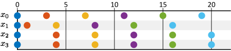
We can use the matrix \({\textrm{\bf{}{T}}}\) to compute the sequence \({\textrm{\bf{}{x}}}(k)\) of concrete time-stamp vectors, of the tokens in the graph, assuming that \({\textrm{\bf{}{x}}}(0)={\bf{0}}\), i.e., that the initial trains all depart at time \(0\). We obtain the following result. \[ {\textrm{\bf{}{x}}}(0)=\begin{bmatrix}{0}\\{0}\\{0}\\{0}\end{bmatrix},~ {\textrm{\bf{}{x}}}(1)=\begin{bmatrix}{3}\\{1}\\{4}\\{4}\end{bmatrix},~ {\textrm{\bf{}{x}}}(2)=\begin{bmatrix}{7}\\{4}\\{8}\\{8}\end{bmatrix},~ {\textrm{\bf{}{x}}}(3)=\begin{bmatrix}{11}\\{8}\\{12}\\{12}\end{bmatrix},~ {\textrm{\bf{}{x}}}(4)=\begin{bmatrix}{15}\\{12}\\{16}\\{16}\end{bmatrix} \]
This states, for example, that the fifth train to leave from Eindhoven to Amsterdam leaves at time 16hrs.
Figure 22 shows the sequence of time-stamp vectors obtained from the matrix \({\textrm{\bf{}{T}}}\) and the initial vector \({\textrm{\bf{}{x}}}(0)={\bf{0}}\).
Reconsider the producer-consumer pipeline of Exercise 13, with function \(f_2\) for the filter actor \(F\). Compute the max-plus matrix for the dataflow graph through symbolic simulation.
Consider the IBC pipeline of Exercise 3.