Dataflow and Max-Plus Algebra

In traditional linear algebra, an important equation to study is the so-called eigenvalue equation. It is also a very important equation for max-plus-linear systems. The equation is as follows. \[ {\textrm{\bf{}{A}}}{\textrm{\bf{}{x}}}=\lambda{}\otimes{}{\textrm{\bf{}{x}}}, |{\textrm{\bf{}{x}}}|\neq{}-\infty{} \](2)

We can read the equation as follows. Given a square matrix \({\textrm{\bf{}{A}}}\), do there exist combinations of a scalar \(\lambda{}\in{}\mathbb{T}\) and a vector \({\textrm{\bf{}{x}}}\), for which Equation 2 holds?

If scalar \(\lambda{}\) and vector \({\textrm{\bf{}{x}}}\) are a solution for the eigenvalue equation for a matrix \({\textrm{\bf{}{A}}}\), then we call \(\lambda{}\) an eigenvalue of \({\textrm{\bf{}{A}}}\) and we call \({\textrm{\bf{}{x}}}\) an eigenvector of \({\textrm{\bf{}{A}}}\). We can easily check that if vector \({\textrm{\bf{}{x}}}\) is an eigenvector of \({\textrm{\bf{}{A}}}\), then also vector \(c\otimes{}{\textrm{\bf{}{x}}}\) is an eigenvector of \({\textrm{\bf{}{A}}}\) for any \(c\in{}\mathbb{T}\) such that \(c\neq{}-\infty{}\). \[ {\textrm{\bf{}{A}}}(c\otimes{}{\textrm{\bf{}{x}}}) = c\otimes{}({\textrm{\bf{}{A}}}{\textrm{\bf{}{x}}}) = c\otimes{}(\lambda{}\otimes{}{\textrm{\bf{}{x}}}) = \lambda{}\otimes{}(c\otimes{}{\textrm{\bf{}{x}}}) \]

Because of this fact, we usually select the eigenvector \({\textrm{\bf{}{x}}}\) with norm \(|{\textrm{\bf{}{x}}}|=0\) as a representative of this class of solutions. Study of the eigenvalue equation is often called spectral analysis.

Observe that the eigenvalue equation only applies to square matrices, since the size of the vector before and after multiplication with the matrix \({\textrm{\bf{}{A}}}\) should be identical. Let matrix \({\textrm{\bf{}{A}}}\), vector \({\textrm{\bf{}{x}}}\) and scalar \(\lambda{}\) be such that the equation holds. Then, the vectors \({\textrm{\bf{}{A}}}{\textrm{\bf{}{x}}}\) and \({\textrm{\bf{}{x}}}\) are similar, each pair of corresponding elements of the vector differ exactly by the amount of \(\lambda{}\).

Example 16 (Dataflow Graph and Eigenvalue Equation)

Consider the matrix \({\textrm{\bf{}{G}}}\) that we derived in Example 13 for the dataflow graph in Figure 20. Note that \({\textrm{\bf{}{G}}}\) is square and may have an eigenvector. Assume that the vector \({\textrm{\bf{}{x}}}\) is an eigenvector of \({\textrm{\bf{}{G}}}\). This means that if we assume that the initial tokens in the dataflow graph are initially available in accordance with the time stamps in the vector \({\textrm{\bf{}{x}}}\), then by conclusion of an iteration of the dataflow graph (i.e., one firing from each of its actors), then the tokens in the graph are reproduced according to the time stamps in the vector \({\textrm{\bf{}{G}}}{\textrm{\bf{}{x}}}=\lambda{}\otimes{}{\textrm{\bf{}{x}}}\). In other words, all tokens in the graph are reproduced exactly \(\lambda{}\) time units after they were initially available. This means that the continued execution of the following iterations of the dataflow graph can continue in a periodic fashion in which for every actor firing \(k+1\) starts exactly \(\lambda{}\) time units after firing \(k\).

A solution to the eigenvalue equation therefore gives us a periodic schedule for the dataflow graph with a known throughput \(\frac{1}{\lambda{}}\) (for any actor). The following equation is a solution to the eigenvalue equation for the matrix \({\textrm{\bf{}{G}}}\). \[ \begin{bmatrix}{-\infty{}}&{0}&{-\infty{}}\\{8}&{-\infty{}}&{7}\\{3}&{-\infty{}}&{2}\\\end{bmatrix} \begin{bmatrix}{-4}\\{0}\\{-5}\end{bmatrix} = 4\otimes{} \begin{bmatrix}{-4}\\{0}\\{-5}\end{bmatrix} = \begin{bmatrix}{0}\\{4}\\{-1}\end{bmatrix} \]

Note that the eigenvector is normal and therefore does not have positive time stamps. The eigenvalue of \({\textrm{\bf{}{G}}}\) is \(\lambda{}=4\). \({\textrm{\bf{}{G}}}\) does not have any other eigenvalues.

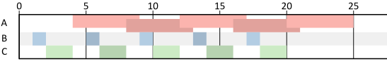
The eigenvalue and eigenvector give rise to a periodic schedule with period \(\lambda{}=4.\) For example, if we assume as the initial time stamps of the initial tokens the eigenvector \(\begin{bmatrix}{1}~{5}~{0}\end{bmatrix}^T\), then we obtain the following periodic schedule. \[ \left\{ \begin{array}{l} \sigma{}(A, k) = 4 + 4k\\ \sigma{}(B, k) = 1 + 4k\\ \sigma{}(C, k) = 2 + 4k\\ \end{array} \right. \]

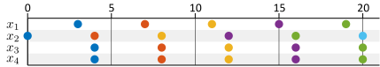
Figure 23 shows a sequence of eigenvectors that represent the evolution of the initial-token time stamps of the dataflow graph of Figure 20 according to this schedule. Figure 24 shows the Gantt chart of the periodic execution of the dataflow graph of Figure 20 according to the schedule \(\sigma{}\). Note that it is indeed periodic.

Example 17 (Railroad Network, Spectral Analysis)

The eigenvalue equation for the railroad network dataflow graph of Figure 7 admits the following solution. \[ \begin{bmatrix} -\infty{} & 1 & 3 & -\infty{} \\ 1 & -\infty{} & -\infty{} & -\infty{} \\ 4 & -\infty{} & -\infty{} & 4 \\ 4 & -\infty{} & -\infty{} & 4 \\ \end{bmatrix} \begin{bmatrix}{-1}\\{-4}\\{0}\\{0}\end{bmatrix} = 4 \otimes{} \begin{bmatrix}{-1}\\{-4}\\{0}\\{0}\end{bmatrix} \]

Assuming that we schedule the initial trains to depart according to the vector \({\textrm{\bf{}{x}}}(0) = \begin{bmatrix}{3}~{0}~{4}~{4}\end{bmatrix}^T\), the trains, under self-timed execution, will assume a periodic schedule. \[ {\textrm{\bf{}{x}}}(0)=\begin{bmatrix}{3}\\{0}\\{4}\\{4}\end{bmatrix}, {\textrm{\bf{}{x}}}(1)=\begin{bmatrix}{7}\\{4}\\{8}\\{8}\end{bmatrix} = 4\otimes{\textrm{\bf{}{x}}}(0), {\textrm{\bf{}{x}}}(2)=\begin{bmatrix}{11}\\{8}\\{12}\\{12}\end{bmatrix} = 8\otimes{\textrm{\bf{}{x}}}(0), {\textrm{\bf{}{x}}}(3)=\begin{bmatrix}{15}\\{12}\\{16}\\{16}\end{bmatrix} = 12\otimes{\textrm{\bf{}{x}}}(0). \]

Figure 27 shows the corresponding periodic sequence of time-stamp eigenvectors with a period equal to the eigenvalue \(\lambda{}=4\).

The largest eigenvalue of a matrix is typically determined by conversion of the matrix to a precedence graph.

Definition 31 (Precedence-Graph Construction)

Given a square matrix \({\textrm{\bf{}{A}}}\in{}\mathbb{T}^{n\times{}n}\), the precedence graph of \({\textrm{\bf{}{A}}}\) is the weighted directed graph with nodes \[ V = \{x_1, \ldots, x_{n}\} \]

The set of weighted edges is defined as follows. \[ E=\lbrace{ (x_j, {\textrm{\bf{}{A}}}[i,j], x_i) } \mid {\textrm{\bf{}{A}}}[i,j]\neq -\infty{} \rbrace{} \]

Definition 32 (Determining the Largest Eigenvalue)

Let \((V,E)\) be the precedence graph of the matrix \({\textrm{\bf{}{A}}}\). The largest eigenvalue of \({\textrm{\bf{}{A}}}\) is equal to the maximum cycle mean (MCM) of the precedence graph. The cycle mean of a cycle is equal to the sum of the weights on all edges of the cycle divided by the number of edges in the cycle. A cycle in the precedence graph with the maximum cycle mean is called a critical cycle of the graph.

Definition 33 (Determining the Eigenvector for the Largest Eigenvalue)

Let \((V,E)\) be the precedence graph of the matrix \({\textrm{\bf{}{A}}}\) and let \(\lambda{}\) be the largest eigenvalue of \({\textrm{\bf{}{A}}}\) and the MCM of the graph. Let \(x_m\) be a node on a critical cycle. Construct the weighted directed graph with nodes \[ V = \{x_1, \ldots, x_{n}\} \]

and the set of weighted edges as follows. \[ E=\lbrace{ (x_j, {\textrm{\bf{}{A}}}[i,j] - \lambda{}, x_i) } \mid {\textrm{\bf{}{A}}}[i,j]\neq -\infty{} \rbrace{}\]

Then an eigenvector \({\textrm{\bf{}{x}}}\) is constructed by taking for \({\textrm{\bf{}{x}}}[k]\) the length of the longest path in the graph from \(x_m\) to \(x_k\). If there is no path from \(x_m\) to \(x_k\) then \({\textrm{\bf{}{x}}}[k]=-\infty{}\)

Note that the weighted directed graph is almost identical to the precedence graph, except that all edge weights have been lowered by \(\lambda{}\). Note further that the resulting eigenvector does not need to be normal (\(|{\textrm{\bf{}{x}}}|\geq{} 0\)). If a normalized eigenvector is desired the resulting vector can easily be normalized afterwards.

Example 18 (Precedence Graph)

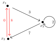
The precedence graph of the matrix from Example 16 is shown in Figure 25. The MCM of the graph is found in the cycle \((x_1, x_2, x_1)\). It has a cycle mean of \(\frac{8}{2}=4\), indeed, the largest eigenvalue of the matrix.

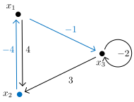
The corresponding eigenvector can be determined from the weighted graph in Figure 26. This is the same graph as the precedence graph, but all edge weights are lowered with the eigenvalue \(\lambda{}=4\). The eigenvector is determined by starting from an arbitrary node \(x_r\) on the critical cycle and determining the longest path in the graph from that node to each of the other nodes in the graph. Note that the graph cannot have any cycles with positive weight since \(\lambda{}\) is the MCM. Therefore the longest path is bounded and in particular does not follow any cycles. The eigenvector \({\textrm{\bf{}{x}}}\) has as its element \({\textrm{\bf{}{x}}}[k]\), the length of the longest path from the root node \(x_r\) to node \(x_k\) if such a path exists and it has the value \(-\infty{}\) if there is no path from \(x_r\) to \(x_k\).

Figure 26 shows the longest paths from root node \(x_2\) in blue and the result is indeed the eigenvector \[ {\textrm{\bf{}{x}}}=\begin{bmatrix}{-4}\\{0}\\{-5}\end{bmatrix} \]

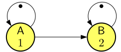
Matrices may have more than one eigenvalue and matrices may also have multiple independent eigenvectors for the same eigenvalue. The following matrix, for example, has two eigenvalues. \[{\textrm{\bf{}{G}}}=\begin{bmatrix}{1} & {-\infty{}}\\{-\infty{}} & {2}\\\end{bmatrix}\] \[{\textrm{\bf{}{G}}}\left[\begin{array}{c}{0}\\{-\infty{}}\\\end{array}\right]= 1\otimes{}\left[\begin{array}{c}{0}\\{-\infty{}}\\\end{array}\right]\] \[{\textrm{\bf{}{G}}}\left[\begin{array}{c}{-\infty{}}\\{0}\\\end{array}\right]= 2\otimes{}\left[\begin{array}{c}{-\infty{}}\\{0}\\\end{array}\right]\]

We may gain some intuition from considering a dataflow graph that corresponds to this matrix, which is the following graph.

It has two actors without mutual dependencies, each proceeds at its own, different pace. This type of graph could also account for the situation of a single eigenvalue with multiple independent eigenvectors. Namely, if the firing duration of actor \(A\) of the above graph would have been 2, both independent vectors would still be eigenvectors, but with a single eigenvalue 2.

Another special case occurs with the matrix of a dataflow graph like the following.

Note that it is similar to the first graph, but now there is a dependency from the actor \(A\) to actor \(B\). Imagine the self-timed execution of the graph. The self-timed schedule is identical to the self-timed schedule of the first graph. With the exception of its first firing, the dependencies of firings of \(B\) on firings of \(A\) are always satisfied by the time the dependency from the self-edge is satisfied.

The corresponding matrix is: \[{\textrm{\bf{}{G}}}=\begin{bmatrix}{1} & {-\infty{}}\\{3} & {2}\\\end{bmatrix}\]

Just like the first graph it has an eigenvalue 2 with the same eigenvector: \[ {\textrm{\bf{}{G}}}\left[\begin{array}{c}{-\infty{}}\\{0}\\\end{array}\right]= 2\otimes{}\left[\begin{array}{c}{-\infty{}}\\{0}\\\end{array}\right] \]

1 is not an eigenvalue of this matrix due to the new dependency. There is, however, a vector, which is strictly speaking not an eigenvector, but has an eigenvector-like property. Consider the vector \({\textrm{\bf{}{x}}}=\left[\begin{array}{c}{-2}\\{0}\\\end{array}\right]\). It is easy to verify that: \[{\textrm{\bf{}{G}}}^k\left[\begin{array}{c}{-2}\\{0}\\\end{array}\right] = \left[\begin{array}{c}{-2+k}\\{2k}\\\end{array}\right]\]

While for a regular eigenvector with eigenvalue \(\lambda\) all elements advance by an amount of \(\lambda\) every time the vector is multiplied by the matrix, in this case all elements of the vector also advance periodically, but with their own rate. In this case the first element advances by 1 and the second element advances by 2. We say that \(\left[\begin{array}{c}{-2}\\{0}\\\end{array}\right]\) is a generalized eigenvector with generalized eigenvalue \(\left[\begin{array}{c}{1}\\{2}\\\end{array}\right]\). A generalized eigenvalue is itself a vector that contains the periods for each of the elements. Such generalized eigenvectors are typical for dataflow graphs in which a fast subgraph produces tokens for a slower subgraph, but there are no dependencies going back.

The Eigenvalue Equation