June, 2022
Linearity of an event system is an important property. It follows directly from the linearity properties that linear event systems allow for a number of convenient analysis techniques. An example is the use of the superposition property, as discussed in the previous section. To further investigate this property we define an event sequence that represents an atomic, individual stimulus. This is the impulse sequence.
The impulse sequence is the event sequence \(\delta{}: \mathbb{N}\rightarrow\mathbb{T}\) such that \(\delta{}(0)=0\) and \(\delta{}(k)=-\infty{}\) for \(k>0\).
The impulse sequence is different from the zero element (\(-\infty{}\)) of the \(\otimes{}\) operator only for the first index \(k=0\), where it is equal to the unit element (\(0\)) of the \(\otimes{}\) operator. Note that the impulse event sequence is a prominent example of an event sequence with decreasing time stamps: \(\delta{}(k)<\delta{}(0)\) for all \(k>0\).
A linear and index-invariant system exposes all of its behavior by its response to the impulse sequence.
The impulse response of an event system \(S\) is the output event sequence \(o\), such that \(\delta{}\mathbin{\stackrel{S}{\longrightarrow}}o\), where \(\delta{}\) is the impulse sequence.
The concept of an impulse response can also be applied to systems with multiple inputs and multiple outputs. The superposition property guarantees us independence also between events on different system inputs. Hence, the impulse response of a system \(S\) on input \(k\) and output \(m\) is \(o_m\) if: \[ \underbrace{\epsilon{}, \ldots{}, \epsilon{}}_{k-1}, \delta{}, \epsilon{}, \ldots, \epsilon{} \mathbin{\stackrel{S}{\longrightarrow}} o_1\ldots{}, o_m, \ldots{}, o_l \]
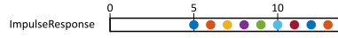
The impulse response of the conveyor belt is the output sequence that corresponds to the input impulse sequence. All objects are present as early as needed (\(-\infty{}\)), except for object 0, which arrives at time 0. Hence, the output sequence, the impulse response of the belt is the sequence \[ h = \left(\frac{l}{v}, \frac{l+d}{v}, \frac{l+2d}{v}, \frac{l+3d}{v}, \ldots{} \right) .\]
The impulse response is shown in Figure 18 for \(l=5\), \(v=1\) and \(d=1\). As all objects following object 0 are placed on the belt as soon as possible, one after the other, after each object a delay of \(\frac{d}{v}\) occurs after which there is room for a new object.
Now imagine a particular arrival of input objects at time stamps \(o_1\), \(o_2\) and \(o_3\). \[(o_1, o_2, o_3, -\infty{}, -\infty{}, \ldots) = o_1\otimes{}\delta{} \oplus{} o_2\otimes{}\delta{}(k-1) \oplus{} o_3\otimes{}\delta{}(k-2)\]
Linearity and index invariance tell us immediately that the corresponding output sequence is \[ a = o_1\otimes{}h \oplus{} o_2\otimes{}h(k-1) \oplus{} o_3\otimes{}h(k-2) .\]
We can write any input sequence \(i\) as a linear combination of delayed impulses as follows: \[ i(k) = \bigoplus_{0\leq{}m\leq{}k } i(m) \otimes{}\delta{}(k-m) = \bigoplus_{0\leq{}m\leq{}k} i(m) \otimes{}{{\delta{}}^{m}}(k) = \bigoplus_{m\geq{}0} i(m) \otimes{}{{\delta{}}^{m}}(k) \]
Hence, \[ i = \bigoplus_{m\geq{}0 } i(m) \otimes{}{{\delta{}}^{m}} \]
Since \(\delta{}\mathbin{\stackrel{S}{\longrightarrow}}h\), by linearity and index invariance, we know that: \[ o = \bigoplus_{m\geq{}0 } i(m) \otimes{}{{h}^{m}} \]
Which means that element \(k\) of the output sequence \(o\) is equal to: \[ o(k) = \bigoplus_{0\leq m \leq{} k } i(m) \otimes{}h(k-m) \](1)
The operation on two event sequences that we recognize on the right-hand side of Equation 1 is called the convolution of the event sequences \(i\) and \(h\). The result of the operation is a new event sequence. It is denoted \(i\otimes{} h\).
Let \(s\) and \(t\) be two event sequences. Their convolution, \(s\otimes{} t\), is the event sequence defined as follows. \[(s\otimes{} t) (k) = \bigoplus_{0\leq{} m\leq{} k} s(m) \otimes{}t(k-m)\]
Note that, by definition of the convolution operation, it is possible to compute a finite prefix (an initial part) of the infinite event sequence that is defined as the convolution of two infinite event sequences from finite prefixes of those event sequences. To compute a prefix of length \(k\) of the convolution, prefixes of length \(k\) of both sequences are needed.
A linear and index-invariant system is entirely defined by its impulse response. No other information about the system is required to determine its output from its input.
If \(S\) is a max-plus-linear and index-invariant system with impulse response \(h\), then for any input event sequence \(i\), \(i\mathbin{\stackrel{S}{\longrightarrow}} i\otimes{} h\).
Note that event with index \(k\) in the convolution does not depend on events with indices larger than \(k\) in either of the functions from which it is computed. This means that in a linear and index-invariant system, output events do not depend on future input events.
The theorem is stated for an event system with a single input and a single output, but it can be easily generalized to multiple inputs and outputs. If \(S\) is a linear and index-invariant event system with \(k\) inputs and \(m\) outputs, with \(h_{l,n}\) the impulse response from input \(l\) to output \(n\), then \[ i_1, \ldots{}, i_k \mathbin{\stackrel{S}{\longrightarrow}} o_1, \ldots{}, o_m \] where for \(1\leq{}n\leq{}m\), \[ o_n = \bigoplus_{l=1}^{k} i\otimes{} h_{l,n} \]

Recall that the railroad network of Examples 5 and 10 can be seen as a max-plus-linear index-invariant event system with as inputs the trains that are arriving from Liège and outputs the trains arriving at Schiphol if we assume that the first trains that do not depend on any input, \(T_1\) through \(T_4\), depart at time \(-\infty{}\). Its impulse response is equal to \[ h_{RR}=[-\infty{}, 6, 10, 14, 18, 22, \ldots] \]
The impulse response is visualized in Figure 19. The \(k\)-th element of an impulse response of a system modeled by a dataflow graph is the duration of the longest path with \(k\) tokens from the respective input to the respective output. If we look at the dataflow graph, we see that there is no path from Liège to Schiphol through channels without tokens. Hence, the first output \(h_{RR}(0)=-\infty{}\) does not depend on the impulse. The initial trains have departed at time \(-\infty{}\) and the first train arrives at the output at \(h_{RR}(0)=-\infty{}\). The second event at the output has time stamp 6. The longest (and only) path from Liège to Schiphol with one token on the path is six hours. It continues in such a way that \(h_{RR}(k) = 2+4k\) for all \(k\geq 1\), the longest path from input to output with \(k\) tokens on it.
Let’s reconsider Example 10. The scheduled arrival times of trains from Liège given in that example are \(l = [0,\) \(5,\) \(10,\) \(15,\) \(20,\) \(25]\). The scheduled arrival times \(s=[4,\) \(8,\) \(12,\) \(16,\) \(21,\) \(26]\) at Schiphol were given assuming self-timed execution and availability of the initial trains \(T_1\) through \(T_4\) at time 0. We can now reconstruct these arrival times analytically, using the above impulse response and, through Theorem 4, convolution. Since the impulse response computed above assumes that initial trains (tokens) have time stamp \(-\infty{}\), we take the effect of the availability of initial trains at time 0 into account through superposition. (Alternatively, we could have transformed the model as explained below Theorem 3. We come back to this alternative in Exercise 12.)
Consider the dataflow graph of Figure 7. Assume all input trains from Liège are available at time \(-\infty{}\) and that the initial trains (tokens) are available at time 0. It is then not difficult to deduce that the arrival times \(s_{st}(k)\) at Schiphol under self-timed execution are \(4+4k\), for \(k\ge 0\).
According to Theorem 4 and using superposition, \(s=l\otimes h_{RR}\oplus s_{st}\). This gives the following results for the arrival times of trains at Schiphol: \[ \begin{array}{ll} s(0) &= (l\otimes h_{RR})(0)\oplus s_{st}(0)\\ &= l(0)\otimes h_{RR}(0)\oplus 4=0\otimes-\infty{}\oplus 4=-\infty{}\oplus 4=4 \\ s(1) &= (l\otimes h_{RR})(1)\oplus s_{st}(1)\\ &= l(0)\otimes h_{RR}(1)\oplus l(1)\otimes h_{RR}(0)\oplus 8=6\oplus-\infty{}\oplus 8=8 \\ s(2) &= (l\otimes h_{RR})(2)\oplus s_{st}(2)\\ &= l(0)\otimes h_{RR}(2)\oplus l(1)\otimes h_{RR}(1)\oplus l(2)\otimes h_{RR}(0)\oplus 12\\ &= 0\otimes 10\oplus 5\otimes 6\oplus 10\otimes-\infty{}\oplus 12=10\oplus 11\oplus-\infty{}\oplus 12=12\\ s(3) &= (l\otimes h_{RR})(3)\oplus s_{st}(3)\\ &= 0\otimes 14\oplus 5\otimes 10\oplus 10\otimes 6\oplus 15\otimes-\infty{}\oplus 16=14\oplus 15\oplus 16\oplus-\infty{}\oplus 16=16\\ s(4) &= (l\otimes h_{RR})(4)\oplus s_{st}(4)\\ &= 0\otimes 18\oplus 5\otimes 14\oplus 10\otimes 10\oplus 15\otimes 6\oplus 20\otimes-\infty{}\oplus 20=21\\ s(5) &= (l\otimes h_{RR})(5)\oplus s_{st}(5)\\ &= 0\otimes 22\oplus 5\otimes 18\oplus 10\otimes 14\oplus 15\otimes 10\oplus 20\otimes 6\oplus 25\otimes-\infty{}\oplus 24=26 \end{array} \] We may observe that initially the availability of the initial trains determines the arrivals at Schiphol, i.e., the maximum is found in \(s_{st}\), whereas the arrival of the last two trains is determined by the input arrivals, the maximum is found in \(l\otimes h_{RR}\).
Reconsider the fragment of the Wireless Channel Decoder (WCD) dataflow model of Exercise 9. In Exercise 10, we showed that this graph specifies a max-plus-linear index-invariant system under a simplifying assumption on the production times of tokens on the self-loop of Actor . We can now compute the self-timed output production times analytically.
We constrain the earliest firing of Actor in self-timed execution to time 0. Theorem 3 states that a dataflow graph with initial tokens available at time \(-\infty{}\) is a max-plus-linear index-invariant system. As explained with Theorem 3 and illustrated with Figure 15 we may consider constraints on the initial token availability in the form of an additional input. We do so in this case with an input called \(sh\) to actor that prevents it from starting earlier than the self-timed execution allows. We moreover assume that the initial token on the self-loop is available at time \(-\infty{}\). We then obtain another max-plus-linear system that is index invariant. Based on Theorem 4, this allows us to compute the (self-timed) output production using convolutions with the impulse responses for each of the inputs. We use indices as in the text earlier to distinguish different impulse responses.