June, 2022
Latency is an important performance property that we can also compute from the state-space representation of a max-plus-linear system. The definition of latency for schedules of dataflow graphs has been defined as the maximum temporal distance among all \(k\in{}\mathbb{N}\) between event \(k\) of an output and event \(k\) of an input. Here, we would like to define latency as an intrinsic property of the system, not just for a particular input sequence. This is not possible, however, without some assumptions about the inputs offered to the system.
We make the following assumptions on input. We will later see that we can relax those assumptions a bit. We assume that all inputs are provided with event sequences \({\textrm{\bf{}{u}}}[k]\) that are periodic with a period \(\mu{}\geq{}\lambda{}\), where \(\lambda{}\) is the largest eigenvalue of the state matrix (i.e., the reciprocal of the maximal throughput of the system). If we offer inputs faster than \(\lambda{}\), then the system will not be able to keep up, the outputs will be produced with a throughput of \(\frac{1}{\lambda{}}\) and the latency will be unbounded. \(\mu{}\) is a parameter of the analysis and the latency result may depend on it. The relation is monotone, however, i.e., a larger period \(\mu{}\) cannot lead to a higher latency.
The latency between input \(i\) and output \(o\) of a max-plus-linear system \(S\) for input period \(\mu{}\) is \[ L(S,\mu{}, i, o) = \bigoplus_{k\in{}\mathbb{N}} y_o(k) - u_i(k) \] where \(u_i\) is the \(\mu{}\)-periodic event sequence (as defined in Definition 14) and \[ \underbrace{\epsilon{}{}, \ldots{}, \epsilon{}{}}_{i-1}, u_i, \epsilon{}{}, \ldots{}, \epsilon{}{} \mathbin{\stackrel{S}{\longrightarrow}} y_1, \ldots{}, y_m\] Since \(u_i\) is \(\mu{}\)-periodic, we have \[ L(S,\mu{}, i, o) = L(y_o, \mu{}) \] where \(L(s, \mu{})\), the \(\mu{}\)-periodic latency of an event sequence \(s\), is defined as \[L(s, \mu{}) = \bigoplus_{k\in{}\mathbb{N}} s(k) - \mu{}\cdot{}k\] this is generalized to a sequence \(\overline{{\textrm{\bf{}{v}}}}\) of vectors as \[L(\overline{{\textrm{\bf{}{v}}}}, \mu{}) = {\textrm{\bf{}{l}}}\] where \[{\textrm{\bf{}{l}}}[k] = L(\overline{{\textrm{\bf{}{v}}}}[k], \mu{})\] I.e., latency is determined for each of the vector elements separately.
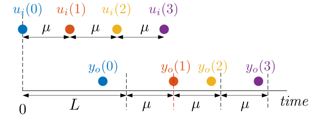
Figure 33 illustrates the definition of latency. The top row shows the \(\mu{}\)-periodic input sequence. The bottom row shows the corresponding output event sequence. In this example, output event \(y_o(1)\) exhibits the maximum latency. The figure also illustrates another interpretation of the latency of system \(S\). If the latency is \(L\) then the output sequence is never later than the \(\mu{}\)-periodic sequence, scaled (i.e., delayed in time) by \(L\). This scaled periodic sequence corresponds to the dashed vertical lines in the figure. The actual outputs are never later.
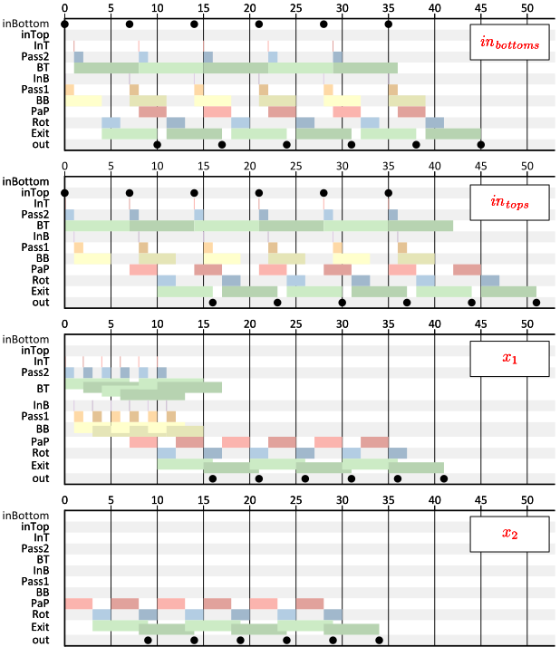
We study the latency of the manufacturing system of Example 2 w.r.t. a desired period \(\mu{}=7\). That is, we would like to compute \(L(\mathit{out}, 7)\). Since \(\lambda{}=5\) (you may wish to check this), we expect it to have a finite latency. The overall latency of the output sequence can be attributed to the combined effect of the input sequences and the elements of the initial state. We can therefore determine the latency from those four contributions separately using the superposition property. We assume that the system is operated from the initial state \({\textrm{\bf{}{x}}}(0)=\begin{bmatrix}{0}~{0}\end{bmatrix}^T\). Figure 34 shows the Gantt charts for each of the four contributing parts separately. The first graph shows the latency due to the \(\mathit{in}_{\mathit{bottom}}\) input. It is the Gantt chart with input \(\mathit{in}_{\mathit{bottom}}\) equal to the \(\mu{}\)-periodic input event sequence and \(\mathit{in}_{\mathit{top}}=\epsilon{}{}\) and with initial state \({\textrm{\bf{}{x}}}(0)=\bf{\epsilon}\). The latency due to the \(\mathit{in}_{\mathit{bottom}}\) input is equal to 10 since all outputs events occur at time \(10+k\cdot\mu{}\).
The second Gantt chart, similarly, shows the latency due to the \(\mathit{in}_{\mathit{top}}\) input. The latency can be seen to be 16. The third Gantt chart investigates the latency due to the first state element, \(x_1\) (the initial token on the edge from actor Pass1 to actor InT in the dataflow graph of Figure 4). Both input sequences are set equal to \(\epsilon{}{}\) and the initial state is set to \({\textrm{\bf{}{x}}}(0)=\begin{bmatrix}{0}~{-\infty{}}\end{bmatrix}^T\). The latency is 16. The maximum value of 16 for \(\mathit{out}(k) - k\cdot\mu{}\) occurs for the first output token (and decreases by 2 for every subsequent output token).
The fourth graph shows that the latency due to the second element, \(x_2\) of the state vector is 9. It is again the first output event that exhibits the largest delay. The Gantt chart starts from the initial state \({\textrm{\bf{}{x}}}(0)=\begin{bmatrix}{-\infty{}}~{0}\end{bmatrix}^T\). Note that since many of the actor firings do not depend on the the second state element (the initial token on the edge Rot—PaP), those actor firings all happen at time stamp \(-\infty{}\) and are therefore not visible in the chart.
The overall latency of the output is therefore equal to the maximum of the four components, \(L(\mathit{out}, 7)=16\).
Latency has been defined, and is analyzed in Example 24, for strictly periodic input sequences with a fixed period \(\mu{}\). We can however exploit the properties of monotonicity and linearity to draw conclusions about the latency of a max-plus-linear and index-invariant system in response to inputs with other, non-periodic patterns too.
Variable and bounded inter-arrival times. If an input event sequence has variable time distance between event arrivals, but a minimum time \(\mu{}\) between any two events, i.e., for all \(k\in{}\mathbb{N}\), \[i(k+1) - i(k) \geq{}\mu{}\] then the latency can be bounded with the latency \(L^{\mu{}}\) of the system for a \(\mu{}\)-periodic input sequence. The argument goes as follows.
The distance between the input \(i\) with the \(\mu{}\)-periodic input is non-decreasing. Let \(\Delta(k)=i(k) - \mu{}\cdot{}k\). Then \(\Delta{}(k+1)\geq{} \Delta{}(k)\) for all \(k\geq{}0\). We know that the output event \(k\) does not depend on any input events with indices larger than \(k\). Therefore, the input \(i\) limited up to event \(k\) produces the same outputs up to event \(k\). Let \(i'\) be the input sequence that includes the events of \(i\) up to and including event \(k\) and let \(i_{\mu{}}\) be the \(\mu{}\)-periodic event sequence up to and including event \(k\). Then \(i'\leq{} \Delta(k)\otimes{}i_{\mu{}}\). Thus, by monotonicity and linearity, \(o(k)\leq{}\Delta{}(k)\otimes{}o_{\mu{}}(k)\), where \(o_{\mu{}}\) is the response to \(i_{\mu{}}\). Thus, \(o(k) - i(k) \leq{} (\Delta{}(k) + o_{\mu{}}(k)) - (i_{\mu{}}(k) + \Delta{}(k)) = o_{\mu{}}(k) - i_{\mu{}}(k) \leq{} L^{\mu{}}\).
Bounded arrival bursts. In a similar way, we can argue that we can determine a bound on the latency of inputs that may arrive in short bursts in which input events temporarily arrive with shorter inter arrival times than \(\mu{}\). Note that this can clearly increase the latency, but we can bound that increase. We need to limit such bursts, because otherwise the latency cannot be bounded. Assume that the input events are such that for all \(k,m\in{}\mathbb{N}\), \(i(m) - i(k)\geq{} (m-k-K)\cdot{}\mu{}\), i.e., up to \(K\) events could arrive simultaneously. Then there exists an input sequence \(i'\) with inter-arrival times bounded by \(\mu{}\), i.e., conforming to the previous case, such that \(i\leq{} i'\leq{} (K\cdot{}\mu{})\otimes{} i\). It is constructed from \(i\) by delaying events that are less than \(\mu{}\) from their predecessor event to be at exactly \(\mu{}\) distance from their predecessor. Let \(o'\) be the output corresponding to \(i'\), then, by monotonicity, \(o\leq{} o'\leq{} (K\cdot{}\mu{})\otimes{} o\). Then \(o(k) -i(k) \leq{} o'(k) - (i'(k) - K\cdot{}\mu{}) \leq{} o'(k)-i'(k) + K\cdot{}\mu{} \leq{} L^{\mu{}}+ K\cdot{}\mu{}.\) Hence, \(L\leq{} L^{\mu{}}+K\cdot{}\mu{}\).
These derivations of latency bounds on different arrival models are due to Moreira (Moreira 2012).
We use the state-space representation of a max-plus-linear system to compute its latency. We start with the observation that the latency \(L\) is influenced by the initial state of the system, as we have seen in Example 24. A larger initial vector may lead to outputs being produced later when they depend on the state. This increases the latency.
Every output of the system has a latency of its own. The latency vector \(L(\overline{{\textrm{\bf{}{y}}}}, \mu{})\) is a vector with the size of the number of outputs and contains as its elements the latencies for each of the outputs. The latency vector can be computed as: \[ L(\overline{{\textrm{\bf{}{y}}}}, \mu{}) = \bigoplus_{k\in{}\mathbb{N}}~ {\textrm{\bf{}{y}}}(k) - k\mu{}\otimes{}{\bf{0}} = \bigoplus_{k\in{}\mathbb{N}}~ (- k\mu{})\otimes{}{\textrm{\bf{}{y}}}(k) ~. \]
Following max-plus-linear-algebra computations (some background details are given below), we can derive that the latency for a max-plus-linear system with state-space matrices \({\textrm{\bf{}{A}}}\), \({\textrm{\bf{}{B}}}\), \({\textrm{\bf{}{C}}}\), and \({\textrm{\bf{}{D}}}\), initial state \({\textrm{\bf{}{x}}}(0)\) and \(\mu{}\)-periodic inputs is computed as follows: \[ \begin{aligned} L(\overline{{\textrm{\bf{}{y}}}}, \mu{}) = {\textrm{\bf{}{C}}}\left({-\mu{}}\otimes{}{\textrm{\bf{}{A}}} \right)^{*} \left( {\textrm{\bf{}{x}}}(0) \oplus \left( {-\mu{}}\otimes{}{\textrm{\bf{}{B}}}{\textrm{\bf{}{0}}} \right) \right) \oplus {\textrm{\bf{}{D}}}{\textrm{\bf{}{0}}} ~, \end{aligned} \](3) where \(\left({-\mu{}}\otimes{}{\textrm{\bf{}{A}}} \right)^{*}\) denotes the so-called \(*\)-closure of the matrix \({-\mu{}}\otimes{}{\textrm{\bf{}{A}}}\). The \(*\)-closure of a square matrix \({\textrm{\bf{}{M}}}\) is defined as \[ \begin{aligned} {\textrm{\bf{}{M}}}^{*} = \bigoplus_{k=0}^{\infty{}} {\textrm{\bf{}{M}}}^k ~. \end{aligned} \]
Note that this closure exists in the latency computation of Equation 3 if and only if the graph has a latency, or, equivalently, if the largest eigenvalue \({\textrm{\bf{}{A}}}\) is not larger than \(\mu{}\). It can be efficiently computed exactly.
The \(*\)-closure of a square matrix \({\textrm{\bf{}{M}}}\in{}\mathbb{T}^{n\times{}n}\) of size \(n\) is defined as follows \[ \begin{aligned} {\textrm{\bf{}{M}}}^{*} = \bigoplus_{k=0}^{\infty{}} {\textrm{\bf{}{M}}}^k ~. \end{aligned} \] It cannot be computed directly following the equation, because it involves the maximum of an infinite number of matrices. One can show however that it is sufficient to compute the maximum of the first \(n\) powers of \({\textrm{\bf{}{M}}}\). \[ \begin{aligned} {\textrm{\bf{}{M}}}^{*} = \bigoplus_{k=0}^{\infty{}} {\textrm{\bf{}{M}}}^k = \bigoplus_{k=0}^{n-1} {\textrm{\bf{}{M}}}^k \end{aligned} \] It is usually computed using the corresponding precedence graph and the observation that the elements of the matrix \({\textrm{\bf{}{M}}}^k\) correspond to the length of the longest path consisting of \(k\) steps between nodes of the precedence graph. Therefore the elements of the \(*\)-closure matrix correspond to the longest paths with an arbitrary number of steps. This can be determined using an all-pairs longest-path algorithm on the precedence graph.
The \(*\)-closure is monotone. I.e., let \({\textrm{\bf{}{A}}}\leq{}{\textrm{\bf{}{B}}}\) such that \({\textrm{\bf{}{B}}}^*\) exists, then \({\textrm{\bf{}{A}}}^*\) exists and \({\textrm{\bf{}{A}}}^*\leq{}{\textrm{\bf{}{B}}}^*\).
As we have seen in Example 24, the latency of a particular output depends on a number of different things, each of the inputs that are needed to produce the output, and the initial state. The principle of superposition tells us however, that the impact of each of these ingredients can be determined completely independently. This is even true for each of the elements, independently, of the initial state vector. We show that therefore, in general, the latency of a system can be characterized by two matrices, namely one, \({\bf{}\Lambda}_{\mathit{IO}}^{\mu{}}\in{}\mathbb{T}^{k\times{}n}\) that contains the latency of every combination of an input and an output, and one, \({\bf{}\Lambda}_{\mathit{state}}^{\mu{}}\in{}\mathbb{T}{{}^{k\times{}m}}\) that contains the latency of every combination of a state vector element with every output, where \(k\) is the number of outputs (length of the output vector), \(n\) is the number of inputs and \(m\) is the length of the state vector.
From the two matrices \({\bf{}\Lambda}_{\mathit{IO}}^{\mu{}}\) and \({\bf{}\Lambda}_{\mathit{state}}^{\mu{}}\), the latency can be computed. For example, the latency from input number \(k\) to output number \(n\) is \[ ({\bf{}\Lambda}_{\mathit{IO}}^{\mu{}}{{\textrm{\bf{}{i}}}_{k}})[n] \] \({\bf{}\Lambda}_{\mathit{IO}}^{\mu{}}{{\textrm{\bf{}{i}}}_{k}}\) gives all output latencies for input \(k\) as a vector, we then pick element \(n\) from the resulting vector.
All output latencies due to the initial state \({\textrm{\bf{}{x}}}(0)\) on output \(k\) are computed as \[ {\bf{}\Lambda}_{\mathit{state}}^{\mu{}}{\textrm{\bf{}{x}}}(0) \]
Latency of a max-plus-linear system. Assume a max-plus-linear system with state-space matrices \({\textrm{\bf{}{A}}}\), \({\textrm{\bf{}{B}}}\), \({\textrm{\bf{}{C}}}\) and \({\textrm{\bf{}{D}}}\). For a given period \(\mu{}\), let vector \({\textrm{\bf{}{l}}}_i = L(\overline{{\textrm{\bf{}{u}}}}, \mu{})\) be a vector of latencies for the inputs \(\overline{{\textrm{\bf{}{u}}}}\).
Then the latency of the outputs \(\overline{{\textrm{\bf{}{y}}}}\) given initial state \({\textrm{\bf{}{x}}}(0)\) and input sequence \(\overline{{\textrm{\bf{}{u}}}}\) for period \(\mu{}\) is equal to \[L{(\overline{{\textrm{\bf{}{y}}}}, \mu{})} = {\bf{}\Lambda}_{\mathit{state}}^{\mu{}}{\textrm{\bf{}{x}}}(0)\oplus{} {\bf{}\Lambda}_{\mathit{IO}}^{\mu{}}{\textrm{\bf{}{l}}}_i\] where \[{\bf{}\Lambda}_{\mathit{state}}^{\mu{}} = {\textrm{\bf{}{C}}}\left({-\mu{}}\otimes{}{\textrm{\bf{}{A}}} \right)^{*}\] \[{\bf{}\Lambda}_{\mathit{IO}}^{\mu{}} = {\bf{}\Lambda}_{\mathit{state}}^{\mu{}} \left( {-\mu{}}\otimes{}{\textrm{\bf{}{B}}} \right) \oplus {\textrm{\bf{}{D}}}\]
Observe that this result conforms to Equation 3 given above.
If we think back of Figure 28 showing the structure of the state-space equations we can find an intuitive interpretation of the equations. The state latency depends on any paths from the state vector to the output. Such a path follows an arbitrary number of iterations through the state matrix \({\textrm{\bf{}{A}}}\) and finally follows the output matrix \({\textrm{\bf{}{C}}}\). Because of the period \(\mu{}\) it gains a delay \(\mu{}\) on every iteration, hence, the \(*\)-closure of the matrix \(-\mu{}\otimes{}{\textrm{\bf{}{A}}}\) finally followed by a multiplication with \({\textrm{\bf{}{C}}}\). Similarly, the equation for the IO latency can be explained. A path from input to output either goes directly via the feed forward matrix \({\textrm{\bf{}{D}}}\), or it goes through the input matrix \({\textrm{\bf{}{B}}}\), then an arbitrary number of iterations on the state matrix, again gaining \(\mu{}\) with every iteration and finally following the output matrix \({\textrm{\bf{}{C}}}\).
We show the derivation of the latency matrices of a max-plus-linear system. The following equation can be shown to hold for the state vector \({\textrm{\bf{}{x}}}(k)\) by induction on \(k\) using the state-space equation \({\textrm{\bf{}{x}}}(k+1) = {\textrm{\bf{}{A}}}{\textrm{\bf{}{x}}}(k) \oplus {\textrm{\bf{}{B}}} {\textrm{\bf{}{u}}}(k)\). \[ {\textrm{\bf{}{x}}}(k) = {\textrm{\bf{}{A}}}^k {\textrm{\bf{}{x}}}(0) \oplus \left( \bigoplus_{m=0}^{k-1} {\textrm{\bf{}{A}}}^m {\textrm{\bf{}{B}}} {\textrm{\bf{}{u}}}(k-m-1) \right) \] Using this result, the output vector can be computed as \[ \begin{aligned} {\textrm{\bf{}{y}}}(k) &= {\textrm{\bf{}{C}}} {\textrm{\bf{}{x}}}(k) \oplus {\textrm{\bf{}{D}}} {\textrm{\bf{}{u}}}(k) \\ &= {\textrm{\bf{}{C}}} \left( {\textrm{\bf{}{A}}}^k {\textrm{\bf{}{x}}}(0) \oplus \bigoplus_{m=0}^{k-1} {\textrm{\bf{}{A}}}^m {\textrm{\bf{}{B}}} {\textrm{\bf{}{u}}}(k-m-1) \right) \oplus {\textrm{\bf{}{D}}} {\textrm{\bf{}{u}}}(k) ~. \end{aligned} \] From this, the output-latency vector \({\textrm{\bf{}{l}}}\) can be computed using the periodic inputs \({\textrm{\bf{}{u}}}(k) = k\cdot\mu{} \otimes{} {\textrm{\bf{}{l}}}_i\) and the definition of latency of a vector sequence. \[ \begin{aligned} {\textrm{\bf{}{l}}}_o &= \bigoplus_{k\in{}\mathbb{N}}~ {\textrm{\bf{}{y}}}(k) - (k\cdot \mu{})\otimes{}{\bf{0}} = \bigoplus_{k\in{}\mathbb{N}}~ (-k\mu{})\otimes{}{\textrm{\bf{}{y}}}(k) \\ &= \bigoplus_{k\in{}\mathbb{N}}~(-k\mu{})\otimes{} {\textrm{\bf{}{C}}} \left({\textrm{\bf{}{A}}}^k {\textrm{\bf{}{x}}}(0)\oplus \bigoplus_{m=0}^{k-1} {\textrm{\bf{}{A}}}^m {\textrm{\bf{}{B}}} {\textrm{\bf{}{u}}}(k-m-1)\right) \oplus {\textrm{\bf{}{D}}} {\textrm{\bf{}{u}}}(k) \\ &= {\textrm{\bf{}{C}}} \bigoplus_{k\in{}\mathbb{N}}~ (-k\mu{})\otimes{}{\textrm{\bf{}{A}}}^{k}{\textrm{\bf{}{x}}}(0) \oplus \\ & \hspace{1.5cm} \bigoplus_{k\in{}\mathbb{N}} (-k\mu{})\otimes{}\left( {\textrm{\bf{}{C}}} \bigoplus_{m=0}^{k-1} \left({\textrm{\bf{}{A}}}^m {\textrm{\bf{}{B}}} (({k-m-1})\cdot\mu{} \otimes{}{\textrm{\bf{}{l}}}_i) \right) \oplus {\textrm{\bf{}{D}}} (k\cdot \mu{} \otimes{} {\textrm{\bf{}{l}}}_i) \right) \\ &= {\textrm{\bf{}{C}}} \bigoplus_{k\in{}\mathbb{N}}~ \left(-\mu{}\otimes{}{\textrm{\bf{}{A}}}\right)^{k}{\textrm{\bf{}{x}}}(0) \oplus \bigoplus_{k\in{}\mathbb{N}} \left( {\textrm{\bf{}{C}}} \bigoplus_{m=0}^{k-1} \left({\textrm{\bf{}{A}}}^m {\textrm{\bf{}{B}}} (({-m-1})\cdot\mu{} \otimes{}{\textrm{\bf{}{l}}}_i ) \right) \oplus {\textrm{\bf{}{D}}} {\textrm{\bf{}{l}}}_i \right) \\ &= {\textrm{\bf{}{C}}} \left(-\mu{}\otimes{}{\textrm{\bf{}{A}}}\right)^*{\textrm{\bf{}{x}}}(0) \oplus {\textrm{\bf{}{C}}} \bigoplus_{k\in{}\mathbb{N}} \left( \bigoplus_{m=0}^{k-1} \left(-\mu{}\otimes{}{\textrm{\bf{}{A}}}\right)^m (-\mu{}) \otimes{}{\textrm{\bf{}{B}}} {\textrm{\bf{}{l}}}_i \right) \oplus {\textrm{\bf{}{D}}} {\textrm{\bf{}{l}}}_i \\ &= {\textrm{\bf{}{C}}} \left(-\mu{}\otimes{}{\textrm{\bf{}{A}}}\right)^*{\textrm{\bf{}{x}}}(0) \oplus {\textrm{\bf{}{C}}} \left( \bigoplus_{m\in{}\mathbb{N}} \left(-\mu{}\otimes{}{\textrm{\bf{}{A}}}\right)^m \right)(-\mu{}) \otimes{}{\textrm{\bf{}{B}}} {\textrm{\bf{}{l}}}_i \oplus {\textrm{\bf{}{D}}} {\textrm{\bf{}{l}}}_i \\ &= {\textrm{\bf{}{C}}} \left(-\mu{}\otimes{}{\textrm{\bf{}{A}}}\right)^*{\textrm{\bf{}{x}}}(0) \oplus {\textrm{\bf{}{C}}} \left(-\mu{}\otimes{}{\textrm{\bf{}{A}}}\right)^*\left(-\mu{} \otimes{}{\textrm{\bf{}{B}}} \right) {\textrm{\bf{}{l}}}_i \oplus {\textrm{\bf{}{D}}} {\textrm{\bf{}{l}}}_i \\ &= {\textrm{\bf{}{C}}} \left(-\mu{}\otimes{}{\textrm{\bf{}{A}}}\right)^*{\textrm{\bf{}{x}}}(0) \oplus \left( {\textrm{\bf{}{C}}} \left(-\mu{}\otimes{}{\textrm{\bf{}{A}}}\right)^*\left(-\mu{} \otimes{}{\textrm{\bf{}{B}}} \right) \oplus {\textrm{\bf{}{D}}} \right) {\textrm{\bf{}{l}}}_i \\ \end{aligned} \]
If we split the result into a part that depends on the initial state and a part that depends on the input latency, we get \[{\textrm{\bf{}{l}}}_o = {\bf{}\Lambda}_{\mathit{state}}^{\mu{}}{\textrm{\bf{}{x}}}(0)\oplus{} {\bf{}\Lambda}_{\mathit{IO}}^{\mu{}}{\textrm{\bf{}{l}}}_i\] where \[{\bf{}\Lambda}_{\mathit{state}}^{\mu{}} = {\textrm{\bf{}{C}}}\left(-\mu{}\otimes{}{\textrm{\bf{}{A}}} \right)^{*}\] \[{\bf{}\Lambda}_{\mathit{IO}}^{\mu{}} = {\textrm{\bf{}{C}}}\left(-\mu{}\otimes{}{\textrm{\bf{}{A}}}\right)^{*} \left( -\mu{}\otimes{}{\textrm{\bf{}{B}}} \right) \oplus {\textrm{\bf{}{D}}} = {\bf{}\Lambda}_{\mathit{state}}^{\mu{}} \left( -\mu{}\otimes{}{\textrm{\bf{}{B}}} \right) \oplus {\textrm{\bf{}{D}}}\]
We continue Example 24. We have in the mean time seen how we can algebraically compute the latency result.
The state-space representation of the manufacturing system can be determined with the methods described in Section 10 with the following outcome. \[ {\textrm{\bf{}{A}}}=\begin{bmatrix}{2} & {-\infty{}}\\{12} & {5}\\\end{bmatrix}, {\textrm{\bf{}{B}}}=\begin{bmatrix}{1} & {2}\\{6} & {12}\\\end{bmatrix} \] \[ {\textrm{\bf{}{C}}}=\begin{bmatrix}{16}~{9}\end{bmatrix}, {\textrm{\bf{}{D}}}=\begin{bmatrix}{10}~{16}\end{bmatrix} \]
We consider latency for the desired period \(\mu{}=7\) as in Example 24. We can now compute the matrices that characterize the latency of the manufacturing system. \[ -\mu{}\otimes{}{\textrm{\bf{}{A}}}=\begin{bmatrix}{-5} & {-\infty{}}\\{5} & {-2}\\\end{bmatrix} \] \[ (-\mu{}\otimes{}{\textrm{\bf{}{A}}})^*=(-\mu{}\otimes{}{\textrm{\bf{}{A}}})^0\oplus(-\mu{}\otimes{}{\textrm{\bf{}{A}}})^1= \begin{bmatrix}{0} & {-\infty{}}\\{-\infty{}} & {0}\\\end{bmatrix} \oplus{} \begin{bmatrix}{-5} & {-\infty{}}\\{5} & {-2}\\\end{bmatrix} =\begin{bmatrix}{0} & {-\infty{}}\\{5} & {0}\\\end{bmatrix} \] Note that in the above computation we have computed the \(*\)-closure using a result that is described in the background discussion on the \(*\)-closure matrix. \[ \begin{aligned} {\bf{}\Lambda}_{\mathit{state}}^{\mu{}} =& {\textrm{\bf{}{C}}}\left(-\mu{}\otimes{}{\textrm{\bf{}{A}}} \right)^{*} \\ =& \begin{bmatrix}{16}~{9}\end{bmatrix} \begin{bmatrix}{0} & {-\infty{}}\\{5} & {0}\\\end{bmatrix} \\ =& \begin{bmatrix}{16}~{9}\end{bmatrix} \end{aligned} \] \[ \begin{aligned} {\bf{}\Lambda}_{\mathit{IO}}^{\mu{}} &= {\bf{}\Lambda}_{\mathit{state}}^{\mu{}} \left( -\mu{}\otimes{}{\textrm{\bf{}{B}}} \right) \oplus {\textrm{\bf{}{D}}} \\ &= \begin{bmatrix}{16}~{9}\end{bmatrix}\begin{bmatrix}{-6} & {-5}\\{-1} & {5}\\\end{bmatrix} \oplus \begin{bmatrix}{10}~{16}\end{bmatrix} = \begin{bmatrix}{10}~{14}\end{bmatrix}\oplus \begin{bmatrix}{10}~{16}\end{bmatrix} \\ &= \begin{bmatrix}{10}~{16}\end{bmatrix} \\ \end{aligned} \]
Note that they indeed give us exactly the four components of the output latency that we could see from the Gantt charts in Figure 34. The latency due to the \(\mathit{in}_{\mathit{bottom}}\) input is 10 (first element of \({\bf{}\Lambda}_{\mathit{IO}}^{\mu{}}\)). The latency due to the \(\mathit{in}_{\mathit{top}}\) input is 16 (second element of \({\bf{}\Lambda}_{\mathit{IO}}^{\mu{}}\)). The latency due to the two initial state elements \(x_1\) and \(x_2\) are 16 and 9 (the elements of \({\bf{}\Lambda}_{\mathit{state}}^{\mu{}}\)), respectively.
From the two matrices, the output latency can be directly computed. Let the initial state be \({\textrm{\bf{}{x}}}(0)=\left[\begin{array}{c}{0}\\{0}\\\end{array}\right]\) and assume that \(\mu{}=7\), that the latency of input sequence \(\mathit{in}_{\mathit{bottom}}\) is 9 and the latency of input sequence \(\mathit{in}_{\mathit{top}}\) is 2, so that \({\textrm{\bf{}{l}}}_i=\left[\begin{array}{c}{9}\\{2}\\\end{array}\right]\). Then, the output latency can be computed as follows. \[ \begin{aligned} L{(\overline{{\textrm{\bf{}{y}}}}, \mu{})} &= {\bf{}\Lambda}_{\mathit{state}}^{\mu{}}{\textrm{\bf{}{x}}}(0)\oplus{} {\bf{}\Lambda}_{\mathit{IO}}^{\mu{}}{\textrm{\bf{}{l}}}_i \\ =& \begin{bmatrix}{16}~{9}\end{bmatrix} \left[\begin{array}{c}{0}\\{0}\\\end{array}\right] \oplus{} \begin{bmatrix}{10}~{16}\end{bmatrix}\left[\begin{array}{c}{9}\\{2}\\\end{array}\right]\\ =& 16 \oplus{} 19 \\ =& 19\\ \end{aligned} \]
It follows directly from the monotonicity properties of max-plus algebra (Section 8), monotonicity of the \(*\)-closure and Equation 3 that latency is monotone in:
Reconsider the IBC pipeline of Exercise 3. Derive the latency \(L(o,4)\) of the output from the state-space model of the IBC pipeline, assuming initial tokens are available at time 0.
Reconsider the wireless channel decoder and its state-space model of Exercise 19. Derive the latency \(L(o,4)\) of the output from the state-space model of the WCD dataflow graph, assuming initial tokens are available at time 0 and assuming 4-periodic input sequences for \(i\) and \(ce\).
Reconsider the producer-consumer pipeline of Exercise 7, with explicit input and output.