June, 2022
Dataflow graphs capture the dependencies between operations in a system and they model how much time the execution of the operations takes. We have seen behaviors of such models, where the actor firings occur as soon as all of their dependency constraints are met. This is, in general, not always the case. The execution may postpone the start of an operation (the firing of the actor in the model) for various reasons, for example, because of limited resource to perform the operations. Dependencies may, however, never be violated. An operation may not occur before all its dependencies are satisfied. In this section, we consider the valid ways that a dataflow graph may be executed and we introduce related performance metrics.
A schedule for a dataflow graph is a (possibly partial) function \(\sigma{}: A\times{}\mathbb{N}\hookrightarrow{}\mathbb{R}\) that assigns starting times to the firings of actors of \(A\), such that \(\sigma{}(a, k)\) is the starting time of firing number \(k\) of actor \(a\). We consider a number of properties that a schedule may have. - The schedule \(\sigma{}\) is called valid for given input arrivals \(\alpha{}: I\times{}\mathbb{N}\hookrightarrow{} \mathbb{R}\) if and only if it satisfies the channel and input constraints:
The schedule that agrees with the Gantt chart of Figure 2 is the following.
\(\sigma{}(A, 0) = 1\), \(\sigma{}(A, 1) = 4\), \(\sigma{}(A, 2) = 7\), \(\sigma{}(A, 3) = 10\), \(\sigma{}(B, 0) = 2\), \(\sigma{}(B, 1) = 5\), \(\sigma{}(B, 2) = 8\), \(\sigma{}(B, 3) = 11\), \(\sigma{}(C, 0) = 2\), \(\sigma{}(C, 1) = 5\), \(\sigma{}(C, 2) = 8\), \(\sigma{}(C, 3) = 11\).
Schedule \(\sigma{}\) is, of course, valid, for the given input. It is also self-timed, and complete, since additional inputs are required to enable further actor firings. \(\sigma{}\) is also periodic, with period 3 and it is finite.
An alap schedule for the output productions \(\pi{}(o,0)=10\), \(\pi{}(o,1)=10\) is the following schedule. \(\sigma{}_l(A, 0) = 2\), \(\sigma{}_l(A, 1) = 5\), \(\sigma{}_l(B, 0) = 3\), \(\sigma{}_l(C, 0) = 6\), \(\sigma{}_l(C, 1) = 6\)
It is valid for the inputs of Figure 2. Note that B only needs to fire once.
A live schedule may not always exist even if infinite input is offered to the dataflow graph. And for a finite number of inputs, a schedule may not exist that consumes all input, i.e., in which all actor firings that depend on that input are assigned a starting time. Graphs for which this applies have deadlocks.
A dataflow graph is said to deadlock if there exist \(a\in{}A\) and \(k\in{}\mathbb{N}\) such that firing \(k\) of actor \(a\) directly or indirectly has a dependency on its own completion.
A single-rate dataflow graph deadlocks if and only if the dataflow graph has a cycle of channel dependencies without initial tokens on them.
A deadlocking single-rate dataflow graph can easily be visually spotted by checking for cycles without initial tokens. For multi-rate dataflow graphs it is less easy. Because it produces and consumes larger quantities of tokens, there may be initial tokens on every cycle, but still not enough for the graph to be free of deadlock. It can be shown however, that a multi-rate dataflow graph is deadlock free if and only if there exists a schedule that assigns start times to all firings in a single iteration of the graph. This can be effectively algorithmically checked.
We take a particular interest in the self-timed schedule of dataflow graphs. We use the property that there cannot be different, but both self-timed schedules.
If a dataflow graph has a self-timed (asap) schedule for input arrivals \(\alpha{}: I\times{}\mathbb{N}\hookrightarrow{} \mathbb{R}\), then it is unique.
Note that the property of Theorem 2 holds true, whether or not we add additional constraints such as an earliest firing time of 0.
With schedules of a dataflow graph we can associate performance metrics. We introduce three metrics in particular. Throughput intuitively refers to the amount of processing that a system can perform, on average, in the long run, per unit of time. It is relevant for indefinite operation. Makespan, in contrast, is a performance metric that can be associated with finite behaviors. It refers to the total amount of time that it takes to complete a job. Finally, latency is a metric that characterizes the time span between the start and the completion of the processing of individual elements. Since this time may differ for different inputs and outputs, latency refers to the maximum difference. Precise definitions are given below.
Given a dataflow graph, an actor \({a}\in{}A\) and a schedule \(\sigma{}\) such that \(\sigma{}(a,k)\) is defined for all \(k\in\mathbb{N}\), the throughput of actor {a} in schedule \(\sigma{}\) is given by the following limit, if it exists: \[ \tau{}(\sigma{},{a}) = \lim_{k\rightarrow{}\infty{}} \frac{k}{\sigma{}({a}, k)} \] Otherwise, the throughput of \(a\) in \(\sigma{}\) is not defined.
If \(\sigma{}\) is a periodic schedule with period \(\mu{}\), then the throughput of any actor, if it fires infinitely often, is equal to \(\frac{1}{\mu{}}\).
Given a dataflow graph with a finite schedule \(\sigma{}\). The makespan of \(\sigma{}\) is \[ M(\sigma{}) = \max_{({a},k)\in{} \mathrm{dom}({\sigma{}})} \sigma{}({a}, k) + e({a}) \]
Given a dataflow graph, input arrivals \(\alpha{}: I\times{}\mathbb{N}\hookrightarrow{}\mathbb{R}\), a selected input \(i\in{}I\) and a selected output \(o\in{}O\) with productions \(\pi{}\) under \(\sigma{}\), let \(K\) be the set of indices for which input on \(i\) and output on \(o\) are defined: \[ K=\lbrace k\in\mathbb{N} \mid (i,k)\in{}\mathrm{dom}({\alpha{}})~\text{and}~(o,k)\in{}\mathrm{dom}({\pi{}}) \rbrace \] then latency is defined as \[ L(\sigma{},i,o) = \sup_{k\in{}K} \pi{}(o, k) - \alpha{}(i,k) \]
In the definition of latency, \(\sup{}\) refers to the supremum, or least upper bound. It is similar to the maximum, but takes care of the situation that there may not exist a unique \(k\) for which the value is the maximum when there are infinitely many \(k\in\mathrm{dom}(\alpha{})\).
Performance metrics are associated with the schedules of the graph. We are often interested in the best possible schedule for a given metric. We can then also associate a performance metric directly with the graph, by which we mean the performance of the best possible schedule. Usually, this is the self-timed schedule. The maximum throughput of a dataflow graph, for example, is the throughput of the self-timed schedule of the graph.
In the schedule of Example 3, the performance metrics are as follows.
It does not have a throughput, because it is a finite schedule. However, if we briefly imagine an infinite periodic continuation of the given schedule, then the throughput of any actor in that schedule is \(\frac{1}{3}\).
The makespan is equal to the time of the latest completion in the schedule, i.e., \(M(\sigma{})= \sigma{}(C,3) +e(C)=15\). The Gantt chart is shown in Figure 2. Makespan can easily be determined from it as the last point in time where there is any activity in the chart.
The latency is equal to the maximum distance between an input and the corresponding output. The largest distance occurs at the last pair of input-output. Therefore, \(L(\sigma{}, i, o) = 15-6 = 9\).
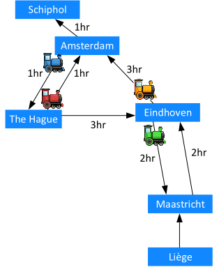
Dataflow is very suitable to model a railroad network. Activities have known durations and there are dependency constraints between operations. Figure 6 shows a small example of a railroad network. The blue rectangles are railroad stations at different cities. We consider the stations Amsterdam, The Hague, Eindhoven and Maastricht to be part of the network we want to model. Trains may be arriving from Liège, which we will consider as inputs to our system and trains may be departing to Schiphol, which we consider as outputs of our system. The railroad trajectories between the stations have known nominal traveling durations as shown in the figure.
Operation of the railroad network needs to comply with certain dependencies. New trains can only depart from a station when all trains that come from neighboring stations have arrived, so as to give the passengers the opportunity to change trains. For simplicity we assume that changing trains does not take any time. To avoid a deadlock, some trains need to initially depart without any trains coming in. We assume there are four trains as shown in the figure.
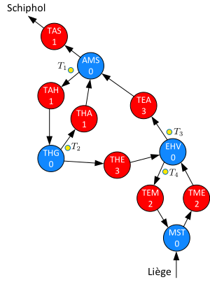
A dataflow graph of the railroad network is shown in Figure 7. The blue actors correspond to the stations. AMS for Amsterdam, THG for The Hague, EHV for Eindhoven and MST for Maastricht. Their input and output dependencies model the synchronization of trains waiting for connection. Their firing durations are equal to \(0\) as we assume that changing trains does not take time. The red colored actors represent the railroad tracks. their firings start when a train departs from the station it consumes from and complete when the train arrives at the next station. Note how the four initial tokens in the graph represent the four trains that initially depart.
Since some of the firings in the dataflow graph do not depend on any inputs, we assume that their earliest starting time in a self-timed execution is equal to 0.
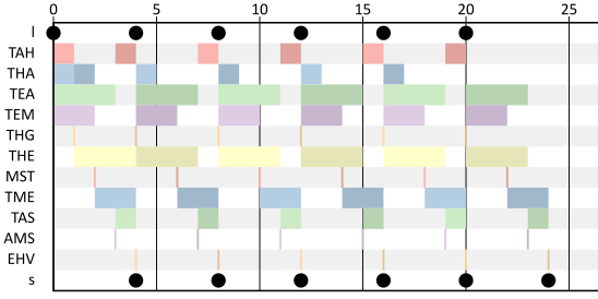
Figure 8 shows a Gantt chart of the self-timed execution of the dataflow graph of the railroad network. After an initial startup phase it assumes a repetitive pattern. The makespan of the schedule is 24hrs. The latency from Liège to Schiphol is 4hrs.
Consider again the Wireless Channel Decoder (WCD) model of Exercise 1. Consider both the options with \(n=1\) and \(n=2\).
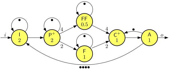
Consider the following variant with explicit inputs and outputs of the producer-consumer pipeline of Exercise 2, with Filter actor F instantiated with filtering function \(f_2\).
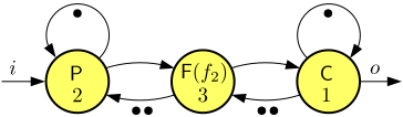
Assume inputs arrive periodically with period 2 and the first input arrives at time 0.
Consider the following variant of the Image-Based Control System (IBCS) of Exercise 5.
Assume inputs arrive periodically with period 2 and the first input arrives at time 0.